A time series is a series of data points, each of which is associated with a time stamp.A simple example is the price of a stock at different times of the day. Another example is the amount of rainfall in an area during different months of the year.

The R language uses many functions to create, manipulate and draw time series data, which is stored in an R object called a time series object.It is also an R data object, such as a vector or a data frame.

Time series objects in R are created using the ts() function with the following syntax:

timeseries.object.name <-  ts(data, start, end, frequency)

The parameters are described as follows:

• data - is a vector or matrix containing the values used in a time series.
• Start - Specifies the start time of the first observation in a time series.
• End - Specifies the end time of the last observation in the time series.
• frequency - Specifies the number of observations per unit time.

These parameters are all optional except the data parameter.

Next, let's make a hypothesis and analyze it step by step.

Suppose that starting in January 2012, we need to present annual rainfall statistics for a location.Then we will create an R time series object for 12 months and draw it as follows:

setwd("D:/r_file")

# Get the data points in form of a R vector.
rainfall <- c(799,1174.8,865.1,1334.6,635.4,918.5,685.5,998.6,784.2,985,882.8,1071)

# Convert it to a time series object.
rainfall.timeseries <- ts(rainfall,start = c(2012,1),frequency = 12)

# Print the timeseries data.
print(rainfall.timeseries)

# Give the chart file a name.
png(file = "rainfall.png")

# Plot a graph of the time series.
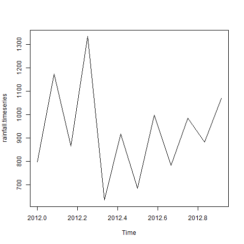
plot(rainfall.timeseries)

# Save the file.
dev.off()

The output is as follows:

Jan    Feb    Mar    Apr    May     Jun    Jul    Aug    Sep
2012  799.0  1174.8  865.1  1334.6  635.4  918.5  685.5  998.6  784.2
        Oct    Nov    Dec
2012  985.0  882.8 1071.0

The resulting pictures are as follows:

The value of the frequency parameter in the ts() function in the above example determines the time interval of the measured data points. The value of 12 indicates that the time series is 12 months. The specific parameters are described as follows:

• frequency= 12 - The data point for each month.
• frequency= 4 - A quarter of the data points per year.
• frequency= 6 - 10 minutes per hour data point.
• Frequency= 246* - 10-minute data points per day.

Finally, let's try to plot multiple time series in a graph, combining the two series into a matrix, as follows:

setwd("D:/r_file")
# Get the data points in form of a R vector.
rainfall1 <- c(799,1174.8,865.1,1334.6,635.4,918.5,685.5,998.6,784.2,985,882.8,1071)
rainfall2 <- 
           c(655,1306.9,1323.4,1172.2,562.2,824,822.4,1265.5,799.6,1105.6,1106.7,1337.8)

# Convert them to a matrix.
combined.rainfall <-  matrix(c(rainfall1,rainfall2),nrow = 12)

# Convert it to a time series object.
rainfall.timeseries <- ts(combined.rainfall,start = c(2012,1),frequency = 12)

# Print the timeseries data.
print(rainfall.timeseries)

# Give the chart file a name.
png(file = "rainfall_combined.png")

# Plot a graph of the time series.
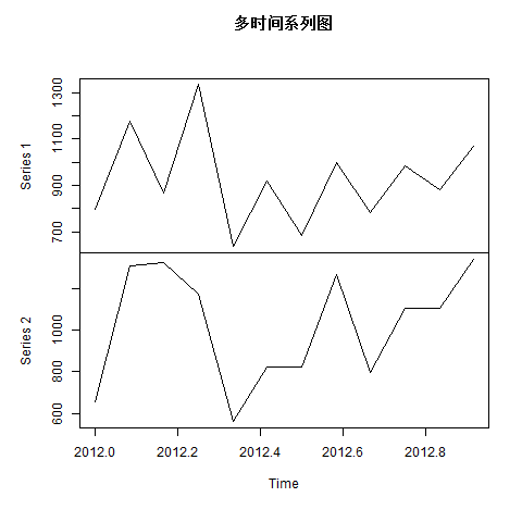
plot(rainfall.timeseries, main = "Multiple Time Series Diagram")

# Save the file.
dev.off()

The output is as follows:

           Series 1  Series 2
Jan 2012    799.0    655.0
Feb 2012   1174.8   1306.9
Mar 2012    865.1   1323.4
Apr 2012   1334.6   1172.2
May 2012    635.4    562.2
Jun 2012    918.5    824.0
Jul 2012    685.5    822.4
Aug 2012    998.6   1265.5
Sep 2012    784.2    799.6
Oct 2012    985.0   1105.6
Nov 2012    882.8   1106.7
Dec 2012   1071.0   1337.8

The resulting pictures are as follows:

Well, that's the record.

If you feel good, please give more support.