Recently, many small data mining projects have been done, using and comparing N-multiple algorithms, and understanding many machine learning tools, such as R language, Spark machine learning library, Python, Tensorflow and RapidMiner, etc. But I feel that I can't go deep into it, at best I just play with other people's tools. The advantages and disadvantages of the algorithm itself and the scope of application are not very much, let alone the improvement of the optimization algorithm.

In the spirit of being a pupil, I recently took part in the course of Machine Learning, which was taught by Andrew Ng, a cattle man of machine learning, at Coursera.( https://www.coursera.org/learn/machine-learning/home/welcome ) This course is the best introductory course that I have ever seen. It is from shallow to deep, step by step. It does not require a deep mathematical foundation and conforms to the natural learning rules. Having just studied for three weeks, I feel I have benefited a lot.
Next, taking the simplest linear regression as an example, the idea of machine learning and its realization in Matlab are briefly introduced.

• 1. Basic concepts
• Hypothesis function
  Hypothesis model (also known as Hypothesis function) is the formula or function that fits the target variable according to the characteristic variable (feature or variable). For example, in the table below, we can estimate the total price of a house from the area of the house according to the hypothetical function, i.e. formula htheta (x) = theta 0 + theta 1*x. This formula is called the hypothetical function, where theta 0 and theta 1 are called parameter s.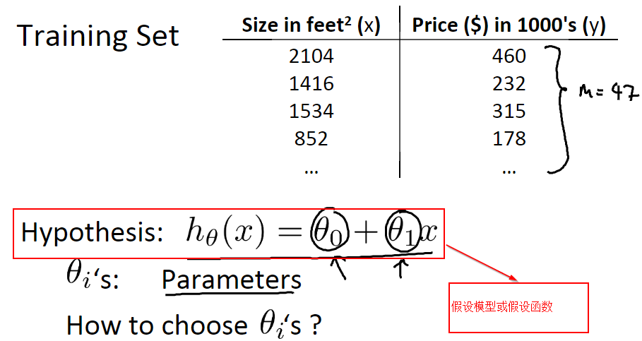
  

The hypothetical models of linear regression are different when different parameters are chosen. The following figure shows three simpler linear regression models.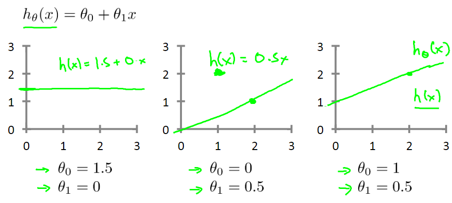

• Cost function
  Cost function or Loss function is used to evaluate the accuracy of hypothesis model fitting. On the training data set, the better the fitting of the model, the smaller the cost function. In machine learning, the purpose of training is to select appropriate parameters (such as theta 0 and theta 1 in the figure above) to minimize the cost function.
  For example, in linear regression, the general definition of the cost function J (theta 0, theta 1) can be understood as the average of the sum of squares of the difference between the real output value of the sample and the estimated value of the hypothetical function as shown in the figure below.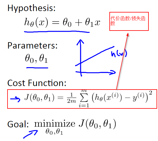
  

• gradient descent
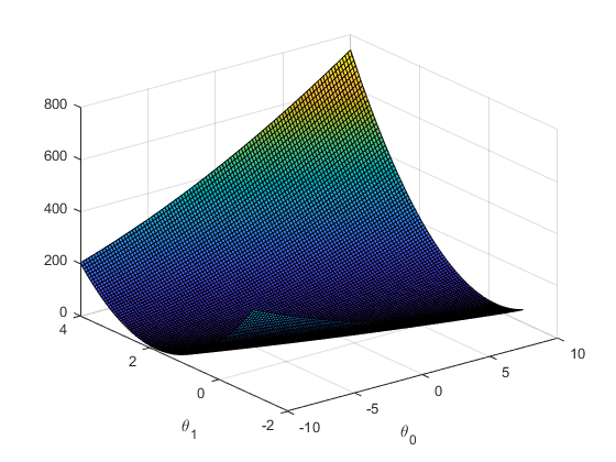
  Gradient descent method is one of the classical methods to minimize the cost function. Previously, I used to use deterministic least square method to find the parameters theta 0 and theta 1 in the hypothetical model h theta(x) = theta 0+theta 1*x, so that the cost function value on the training set was minimized. In fact, the cost function J (theta 0, theta 1) can be regarded as a function composed of two variables theta 0 and theta 1. The visualization result of this function is shown in the following figure. The goal of our study is to find the appropriate theta 0 and theta 1 in the graph, so that J (theta 0, theta 1) can approach and reach the local or global minimum (the point in the red circle in the figure below).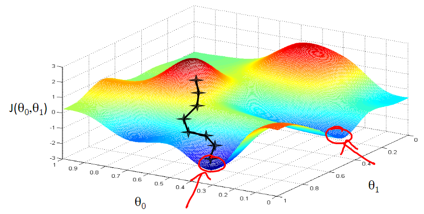
  

An intuitive explanation of the gradient descent in the picture is: "For example, somewhere on a big mountain, because we don't know how to get down, we decided to take one step at a time. That is, when we get to a position, we will solve the gradient of the current position, and go down along the negative direction of the gradient, that is, the steepest position at present, and then continue to solve the problem." Forward position gradient, take a step to the position where this step is located along the steepest and easiest downhill position. Step by step, until we feel that we have reached the foot of the mountain. Of course, if we go on like this, maybe we can't go to the foot of the mountain, but to some part of the low peak. ( http://www.cnblogs.com/pinard/p/5970503.html ) Gradient descent method is not only suitable for linear regression, but also can be used in logical regression and other algorithms.

Geometrically, given an arbitrary starting point (theta 0, theta 1) on the surface of the cost function J (theta 0, theta 1), we can iterate continuously along the direction of gradient descent, i.e., the direction of partial derivatives of theta 0 and theta 1 in the cost function J (theta 0, theta 1) according to a certain step size (a, learning rate, learning efficiency), until theta 0 and theta 1 converge, that is to say, the direction of partial derivatives in the cost function J (theta 0, theta 1). Local or global minimum. For a simple linear regression, the algorithm is described as follows: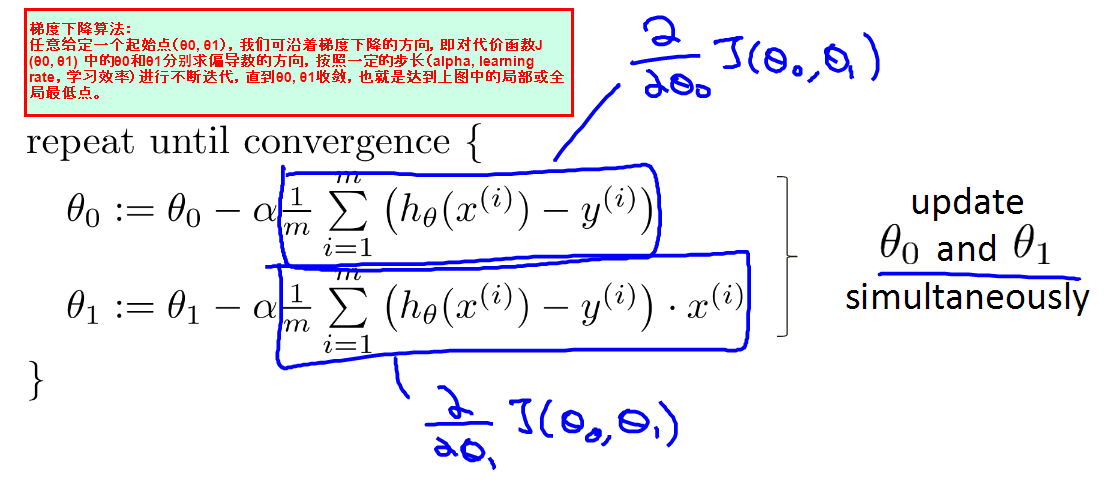

• 2. Simple implementation
  In Matlab or Octave, we can simply realize linear regression by the principle of loss function and gradient descent.

Assuming that the original data are as follows, x denotes the population of the city and y represents the profit of the city. We can use the population of a city to predict its profit by linear regression. The detailed code is as follows:

%% stay Matlab Or Octave Gradient descent method and linear regression
%% Initialization
clear ; close all; clc;
%%Loading data
% x Indicate the number of people in a city.
x = [6.1101; 5.5277; 8.5186; 7.0032; 5.8598; 8.3829; 7.4764; 8.5781; 6.4862; 5.0546; 5.7107; 14.1640; 5.7340; 8.4084; 5.6407; 5.3794; 6.3654; 5.1301; 6.4296; 7.0708; 6.1891; 20.2700; 5.4901; 6.3261; 5.5649; 18.9450; 12.8280; 10.9570; 13.1760; 22.2030; 5.2524; 6.5894; 9.2482; 5.8918; 8.2111; 7.9334; 8.0959; 5.6063; 12.8360; 6.3534; 5.4069; 6.8825; 11.7080; 5.7737; 7.8247; 7.0931; 5.0702; 5.8014; 11.7000; 5.5416; 7.5402; 5.3077; 7.4239; 7.6031; 6.3328; 6.3589; 6.2742; 5.6397; 9.3102; 9.4536; 8.8254; 5.1793; 21.2790; 14.9080; 18.9590; 7.2182; 8.2951; 10.2360; 5.4994; 20.3410; 10.1360; 7.3345; 6.0062; 7.2259; 5.0269; 6.5479; 7.5386; 5.0365; 10.2740; 5.1077; 5.7292; 5.1884; 6.3557; 9.7687; 6.5159; 8.5172; 9.1802; 6.0020; 5.5204; 5.0594; 5.7077; 7.6366; 5.8707; 5.3054; 8.2934; 13.3940; 5.4369];
% y On behalf of the profits of the city
y = [ 17.5920;9.1302;13.6620;11.8540;6.8233;11.8860;4.3483;12.0000;6.5987;3.8166;3.2522;15.5050;3.1551;7.2258;0.7162;3.5129;5.3048;0.5608;3.6518;5.3893;3.1386;21.7670;4.2630;5.1875;3.0825;22.6380;13.5010;7.0467;14.6920;24.1470;-.2200;5.9966;12.1340;1.8495;6.5426;4.5623;4.1164;3.3928;10.1170;5.4974;0.5566;3.9115;5.3854;2.4406;6.7318;1.0463;5.1337;1.8440;8.0043;1.0179;6.7504;1.8396;4.2885;4.9981;1.4233;-1.4211;2.4756;4.6042;3.9624;5.4141;5.1694;-0.7428;17.9290;12.0540;17.0540;4.8852;5.7442;7.7754;1.0173;20.9920;6.6799;4.0259;1.2784;3.3411;-.6807;0.2968;3.8845;5.7014;6.7526;2.0576;0.4795;0.2042;0.6786;7.5435;5.3436;4.2415;6.7981;0.9270;0.1520;2.8214;1.8451;4.2959;7.2029;1.9869;0.1445;9.0551;0.6170];
% m Is the number of training samples
m = length(y);
%% Yes x, y Drawing
% Data points are represented by a cross symbol with a size of 10
plot(x, y, 'rx', 'MarkerSize', 10);
% Set up X axis
xlabel('population');
% Set up Y axis
ylabel('profit');

Then, we can create a new computeCost.m file in the current working directory, which contains only one computeCost function to calculate the value of the cost function. The code is as follows:

function J = computeCost(X, y, theta)
%COMPUTECOST Compute cost for linear regression
%   J = COMPUTECOST(X, y, theta) computes the cost of using theta as the
%   parameter for linear regression to fit the data points in X and y

% Initialize some useful values
m = length(y); % number of training examples

% You need to return the following variables correctly 
J = 0;

hypothesis = X * theta;
J = sum((hypothesis - y) .^ 2);
J = J/(2*m);

% =========================================================================
end

Similarly, we can create another gradient Descent. m file in the current working directory, which contains only one gradient Descent function to iterate gradient descent according to the number of iterations and the alpha (learning efficiency) set. Finally, we visualize the results of linear regression. The code is as follows:

function [theta, J_history] = gradientDescent(X, y, theta, alpha, num_iters)
%GRADIENTDESCENT Performs gradient descent to learn theta
%   theta = GRADIENTDESCENT(X, y, theta, alpha, num_iters) updates theta by 
%   taking num_iters gradient steps with learning rate alpha

% Initialize some useful values
m = length(y); % number of training examples
J_history = zeros(num_iters, 1);

temp = zeros(2, 1);

for iter = 1:num_iters

    hypothesis = X * theta -  y;
    n = length(theta);
    for j = 1:n
        theta(j) = theta(j) - alpha/m * (hypothesis' * X(:,j));
    end

    % ============================================================
    % Save the cost J in every iteration    
    J_history(iter) = computeCost(X, y, theta);

    %fprintf('the cost is %f\n', J_history(iter));

end

end

After writing these two functions, we can calculate the value of the cost function and use gradient descent iteration method to make linear regression. See the code specifically:

%% =================== Calculating cost function and gradient descent iteration ===================
% stay x The vector is preceded by a column of m A vector of one, a vector of one. X matrix
X = [ones(m, 1), x]; % Add a column of ones to x
% Initialization theta parameter
theta = zeros(2, 1); % initialize fitting parameters

% The number of iterations of gradient descent is 1500 and the learning rate step is long. alpha For 0.01；If it does not converge, the step size can be reduced.
iterations = 3000;
alpha = 0.01;
fprintf('\n Test Cost Function ...\n')
% Calculating the value of the initial cost function
J = computeCost(X, y, theta);
fprintf('With theta = [0 ; 0]\nCost computed = %f\n', J);
fprintf('Expected cost value (approx) 32.07\n');

fprintf('\n Start gradient descent iteration ...\n')
% run gradient descent
theta = gradientDescent(X, y, theta, alpha, iterations);

% print theta to screen
fprintf('Theta found by gradient descent:\n');
fprintf('%f\n', theta);
fprintf('Expected theta values (approx)\n');
fprintf(' -3.6303\n  1.1664\n\n');

% Plot the linear fit
hold on; % keep previous plot visible
plot(X(:,2), X*theta, '-')
legend('Training data', 'Linear regression')
hold off % don't overlay any more plots on this figure

% According to the fitting linear regression curve, the population is 35.,000 And 70,000 The profits of the two cities are forecasted.
predict1 = [1, 3.5] *theta;
fprintf('For population = 35,000, we predict a profit of %f\n',...
    predict1*10000);
predict2 = [1, 7] * theta;
fprintf('For population = 70,000, we predict a profit of %f\n',...
    predict2*10000);

fprintf('Program paused. Press enter to continue.\n');


%% ============= visualization J(theta_0, theta_1) =============
fprintf('Visualizing J(theta_0, theta_1) ...\n')

% Grid over which we will calculate J
theta0_vals = linspace(-10, 10, 100);
theta1_vals = linspace(-1, 4, 100);

% initialize J_vals to a matrix of 0's
J_vals = zeros(length(theta0_vals), length(theta1_vals));

% Fill out J_vals
for i = 1:length(theta0_vals)
    for j = 1:length(theta1_vals)
      t = [theta0_vals(i); theta1_vals(j)];
      J_vals(i,j) = computeCost(X, y, t);
    end
end


% Because of the way meshgrids work in the surf command, we need to
% transpose J_vals before calling surf, or else the axes will be flipped
J_vals = J_vals';
% Surface plot
figure;
surf(theta0_vals, theta1_vals, J_vals)
xlabel('\theta_0'); ylabel('\theta_1');

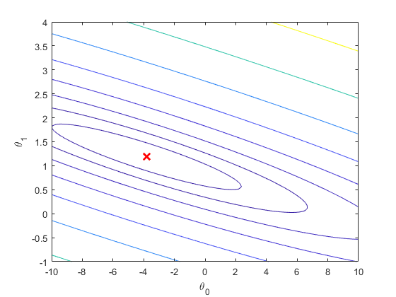
% Contour plot
figure;
% Plot J_vals as 15 contours spaced logarithmically between 0.01 and 100
contour(theta0_vals, theta1_vals, J_vals, logspace(-2, 3, 20))
xlabel('\theta_0'); ylabel('\theta_1');
hold on;
plot(theta(1), theta(2), 'rx', 'MarkerSize', 10, 'LineWidth', 2);

The visualization results are as follows: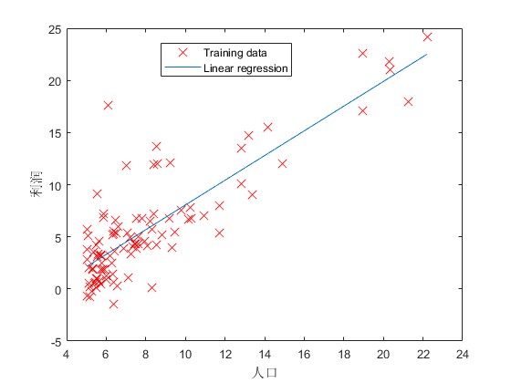

• Reference
  Coursera Machine Learning, Programming Ex.1, https://www.coursera.org/learn/machine-learning/resources/O756o
  Coursera Machine Learning, Week 1 Lecture notes, https://www.coursera.org/learn/machine-learning/resources/JXWWS
  Liu Jianping, 2016, Summary of Gradient Descent, http://www.cnblogs.com/pinard/p/5970503.html