This paper introduces Topsis comprehensive evaluation method, illustrates its calculation process through a practical case, and realizes it by using R language.

1. Overview of TOPSIS method

The full name of TOPSIS is technology for order preference by similarity to an ideal solution. TOPSIS method was first proposed by C.L.Hwang and K.Yoon in 1981. It is a method of ranking according to the proximity between a limited number of evaluation objects and idealized objectives. It is to evaluate the relative advantages and disadvantages of existing objects. As a ranking method approaching the ideal solution, this method only requires that each utility function be monotonically increasing (or decreasing). It is a commonly used and effective method in multi-objective decision analysis, also known as the good and bad solution distance method.

The basic idea of this method is: Based on the normalized original data matrix, the cosine method is used to find the optimal scheme and the worst scheme in the limited scheme (expressed by the optimal vector and the worst vector respectively), and then the distance between each evaluation object and the optimal scheme and the worst scheme is calculated respectively to obtain the relative proximity between each evaluation object and the optimal scheme, As the basis for evaluating the advantages and disadvantages.

2. Sample data

An epidemic prevention station plans to evaluate the quality of health supervision in local public places from 1997 to 2001
The price index includes supervision rate% (x1), physical examination rate% (x2) and training rate% (x3). The original data are as follows:

   year  idx1  idx2  idx3
 1997  95    95.3  95  
 1998 100    90    90.2
 1999  97.4  97.5  94.6
 2000  98.4  98.2  90.3
 2001 100    97.4  92.5

Now it is necessary to comprehensively evaluate the quality of health supervision in public places for five years.

R implementation process

1. Load data and package

library(dplyr)
library(readr)
# load sample data
dat <- read_csv("data/sample.csv")

2. Normalization

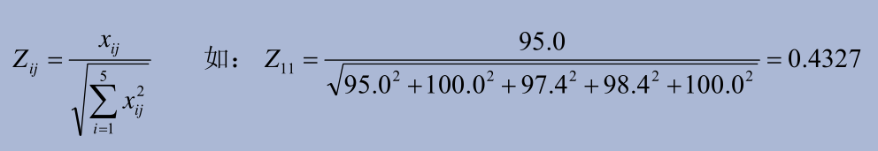
# Standardized variable value function
z_value <- function(x){
  x / sqrt(sum(x^2))
}

# Standardize data by column
dat_z <- dat %>% mutate(across(c(2:4), z_value))

# Return normalized data matrix
# year  idx1  idx2  idx3
# 1997 0.433 0.445 0.459
# 1998 0.456 0.420 0.436
# 1999 0.444 0.455 0.457
# 2000 0.448 0.459 0.436
# 2001 0.456 0.455 0.447

3. Determine the best scheme and the worst scheme

The optimal scheme Z + consists of the maximum value in each column in Z: Z + = (maxz I1, maxz I2,..., maxZ im)
Worst case Z - consists of the minimum value in each column in Z: Z + = (Minz I1, Minz I2,..., minZ im)

## unlist converts tibble to vector
z_max <- dat_z %>% summarise(across(c(2:4), max)) %>% unlist
# > z_max
# idx1      idx2      idx3 
# 0.4555144 0.4587666 0.4590897 

z_min <- dat_z %>% summarise(across(c(2:4), min)) %>% unlist
# > z_min
# idx1      idx2      idx3 
# 0.4327386 0.4204582 0.4358936 

4. Calculate the optimal D + and the worst D of the distance between each evaluation object and Z + and Z --

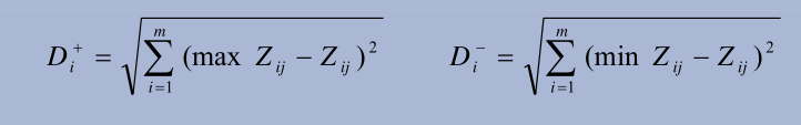
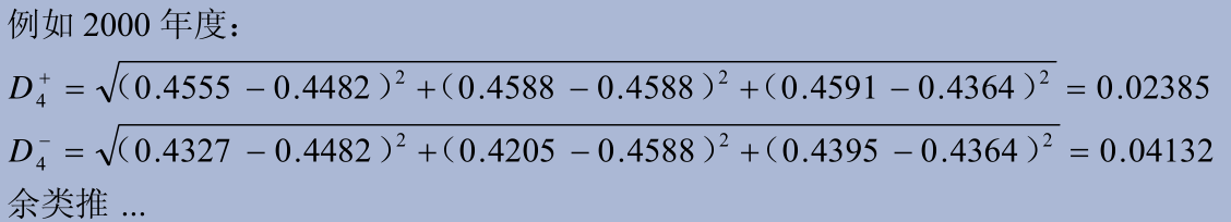
# Calculate distance
dist <-function(x, std){
  res <- c()
  for ( i in 1 : nrow(x)) {
    res[i] = sqrt(sum((unlist(x[i,-1])-std)^2))
  }
  
  return(res)
}

# Optimal distance D+
du <- dist(dat_z, z_max)
# Worst distance D-
dn <- dist(dat_z, z_min)

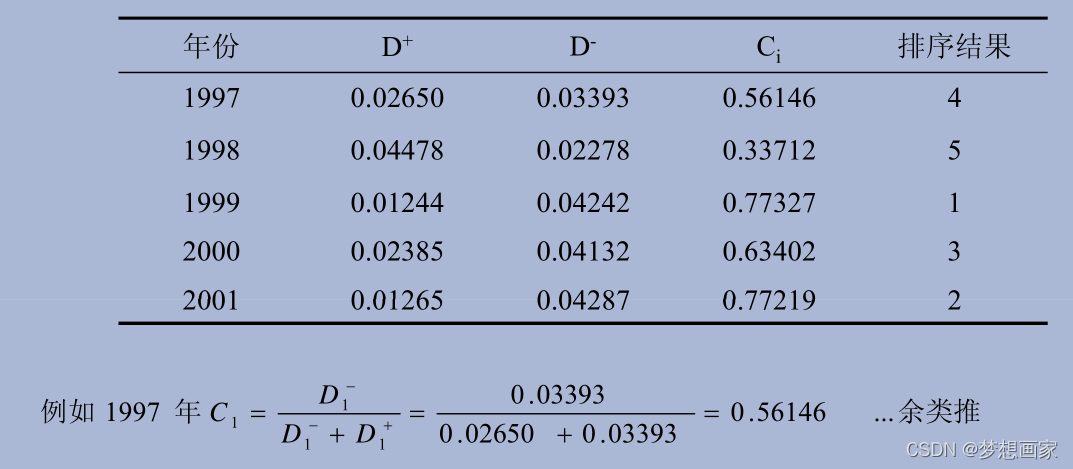
5. Calculate the proximity Ci between each evaluation object and the optimal scheme

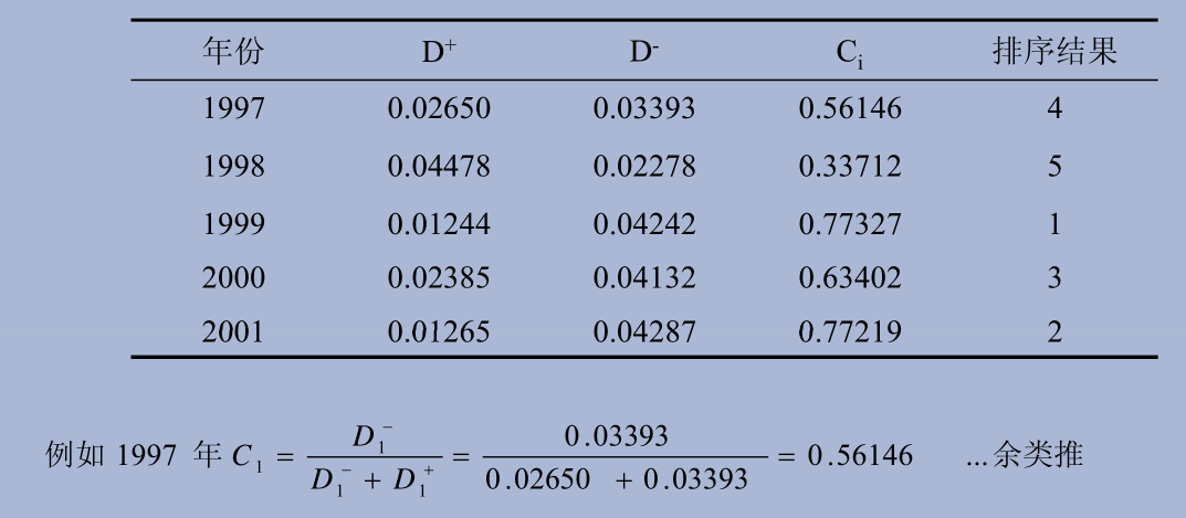
Implementation code:

# CI S are calculated and sorted in descending order
dat_z %>% add_column(du = du, dn = dn) %>% 
      mutate(ci= dn/(du+dn)) %>%
      arrange(-ci)
 # The final returned result is:
 # year  idx1  idx2  idx3     du     dn    ci
# 1999 0.444 0.455 0.457 0.0124 0.0424 0.773
# 2001 0.456 0.455 0.447 0.0126 0.0429 0.772
# 2000 0.448 0.459 0.436 0.0239 0.0413 0.634
# 1997 0.433 0.445 0.459 0.0265 0.0339 0.561
# 1998 0.456 0.420 0.436 0.0448 0.0228 0.337

6. Complete process

The complete code is given below:

library(dplyr)
library(readr)

# Normalized variable value
z_value <- function(x){
  x / sqrt(sum(x^2))
}

# Calculate the optimal distance
dist <-function(x, std){
  res <- c()
  for ( i in 1 : nrow(x)) {
    res[i] = sqrt(sum((unlist(x[i,-1])-std)^2))
  }
  
  return(res)
}

# load sample data
dat <- read_csv("data/sample.csv")

# Standardize data by column
dat_z <- dat %>% mutate(across(c(2:4), z_value))

## unlist converts tibble to vector
z_max <- dat_z %>% summarise(across(c(2:4), max)) %>% unlist
z_min <- dat_z %>% summarise(across(c(2:4), min)) %>% unlist

# dat_z %>% select(2:4) %>% rowwise() %>% mutate(du = dist(., z_max), dn= dist(., z_min)) 
du <- dist(dat_z, z_max)
dn <- dist(dat_z, z_min)

# CI S are calculated and sorted in descending order
dat_z %>% add_column(du = du, dn = dn) %>% 
      mutate(ci= dn/(du+dn)) %>%
      arrange(-ci)