from Last article The analysis has learned that the golden cross rule of the mean line does not apply to the concussion period, so what is the way to avoid the concussion period or what is the way to reduce the loss of no brain following? Let's keep playing.

Required Packages

library(quantmod)
library(ggplot2)
library(scales)

Postpone Trading

The first way to try is to postpone the buying time.

If the stock price is in a period of volatility, it is possible that it will rise today and fall tomorrow. We can temporarily suppress the impulse of buying when the buying signal appears, and postpone for 3-5 days to see if the stock price is still rising. If so, let's be bold.

get_signals <- function(data, mas_1=5, mas_2=20, delay_days= 3) {
  if(mas_1 == 0)
    ma_name_1 <- "Value"
  else
    ma_name_1 <- paste('MA', mas_1, sep='')
  ma_name_2 <- paste('MA', mas_2, sep='')
  ma_data <- data[, c("Value", ma_name_1, ma_name_2)]
  signals <- data.frame(Index=index(ma_data), coredata(ma_data))
  signals$Trade <- ifelse(signals[,c(ma_name_1)] > signals[,c(ma_name_2)], 1, 0)
  signals <- signals[-c(1:mas_2),]
  signals$Signal <- c(signals$Trade[1],diff(signals$Trade))
  signals$Diff_1 <- c(NA, diff(signals[,c(ma_name_1)]))
  signals$Diff_2 <- c(NA, diff(signals[,c(ma_name_2)]))
  ######
  buy <- which(signals$Signal == 1)
  sell <- which(signals$Signal == -1)
  for(ii in 1:length(buy)){
    tmp <- 0
    index <- buy[ii]
    signals$Signal[index] <- 0
    for(jj in 1:delay_days) 
      tmp <- tmp + signals$Trade[index + jj]
    if(tmp == delay_days) 
      signals$Signal[index + delay_days] <- 1
    else
      signals$Signal[sell[ii]] <- 0
  }
  ######
  signals <- signals[which(signals$Signal != 0),]

  if(nrow(signals)%%2 == 1) {
    if(signals$Trade[1] == 1)
      signals <- signals[-c(nrow(signals)),]
    else
      signals <- signals[-c(1),]
  }
  if(signals$Trade[1] == 0) {
    signals <- signals[-c(nrow(signals)),]
    signals <- signals[-c(1),]
  }
  signals <- signals[,-which(names(signals)%in% c(ma_name_1, ma_name_2, "Diff_1", "Diff_2"))]
  return (signals)
}

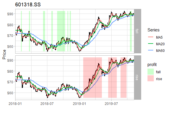
If we delay 3 days when the buying signal appears and the short-term average is still higher than the long-term average within these 3 days, then we will buy. So from January 1, 2018 to November 7, 2019 (the deadline of the last analysis), there are 22 transactions (total transactions), which is 8 fewer than that in the previous analysis. The principal was 92293.10 and the loss was 7706.90. The loss rate dropped from 19% to 7%. In addition, we can see from the figure that delayed buying also reduced frequent trading in 2018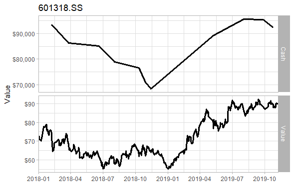

Early Termination

The second way is to terminate the transaction in advance, commonly known as stop loss.

We can set a stop line, that is, when the stock price falls below a certain position, whether it is a dead gold cross or not, we will sell it and stop the loss immediately.

get_signals <- function(data, mas_1=5, mas_2=20, sell_ratio = 0.05) {
  if(mas_1 == 0)
    ma_name_1 <- "Value"
  else
    ma_name_1 <- paste('MA', mas_1, sep='')
  ma_name_2 <- paste('MA', mas_2, sep='')
  ma_data <- data[, c("Value", ma_name_1, ma_name_2)]
  signals <- data.frame(Index=index(ma_data), coredata(ma_data))
  signals$Trade <- ifelse(signals[,c(ma_name_1)] > signals[,c(ma_name_2)], 1, 0)
  signals <- signals[-c(1:mas_2),]
  signals$Signal <- c(signals$Trade[1],diff(signals$Trade))
  signals$Diff_1 <- c(NA, diff(signals[,c(ma_name_1)]))
  signals$Diff_2 <- c(NA, diff(signals[,c(ma_name_2)]))
  #####
  buy <- which(signals$Signal == 1)
  sell <- which(signals$Signal == -1)
  iteration <- min(length(buy), length(sell))
  if(sell_ratio > 0) {
    for(ii in 1:iteration){
      buy_index <- buy[ii]
      sell_index <- sell[ii]
      for(jj in buy_index:sell_index){
        if(signals$Value[jj]/signals$Value[buy_index] > 1 + sell_ratio | signals$Value[jj]/signals$Value[buy_index] < 1- (sell_ratio - 0.02)) {
          signals$Signal[sell_index] <- 0
          signals$Signal[jj] <- -1
          signals$Trade[jj] <- 0
          break
        }
      }
    }
  }
  #####
  signals <- signals[which(signals$Signal != 0),]

  if(nrow(signals)%%2 == 1) {
    if(signals$Trade[1] == 1)
      signals <- signals[-c(nrow(signals)),]
    else
      signals <- signals[-c(1),]
  }
  if(signals$Trade[1] == 0) {
    signals <- signals[-c(nrow(signals)),]
    signals <- signals[-c(1),]
  }
  signals <- signals[,-which(names(signals)%in% c(ma_name_1, ma_name_2, "Diff_1", "Diff_2"))]
  return (signals)
}

Let's say we set the stop loss at 7%, i.e. if it's less than 7% of the buying price, we'll sell. From January 1, 2018 to November 7, 2019 (the deadline of the last analysis), there are 30 transactions (total sales) and 6 profitable transactions. The final principal was 84796.95, with a loss of 15203.05. The loss rate dropped from 19% to 15%.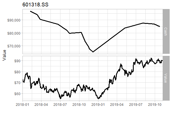

Differentiate

We all know that the average is delayed. We can't predict 100% whether it's in the shock period at this time. But in general, the average in the period of shock tends to be flat (i.e. the slope is close to zero), while the average in the period of trend is inclined, and the more inclined (the larger the slope), the larger the space for rising. It is more accurate to judge the performance with long-term average.

We use the slope of the average to filter some buying points that show a gentle trend, that is, we can only buy when the buying signal appears and the slope of the average at this time is greater than a certain value, otherwise, we will not trade.

get_signals <- function(data, mas_1=5, mas_2=20, filter_type=0) {
  if(mas_1 == 0)
    ma_name_1 <- "Value"
  else
    ma_name_1 <- paste('MA', mas_1, sep='')
  ma_name_2 <- paste('MA', mas_2, sep='')
  ma_data <- data[, c("Value", ma_name_1, ma_name_2)]
  signals <- data.frame(Index=index(ma_data), coredata(ma_data))
  signals$Trade <- ifelse(signals[,c(ma_name_1)] > signals[,c(ma_name_2)], 1, 0)
  signals <- signals[-c(1:mas_2),]
  signals$Signal <- c(signals$Trade[1],diff(signals$Trade))
  signals$Diff_1 <- c(NA, diff(signals[,c(ma_name_1)]))
  signals$Diff_2 <- c(NA, diff(signals[,c(ma_name_2)]))
  signals <- signals[which(signals$Signal != 0),]

  #####
  switch(filter_type,
         "NO_FILTER" = print("No Filter!"),
         "DIFF_SHORTTERM_GREATER_THAN_POINT_5" = signals <- signals[-c(which(signals$Signal == 1 & signals$Diff_1 < 0.5), 
                                                                    which(signals$Signal == 1 & signals$Diff_1 < 0.5) + 1),]
  )
  #####

  if(nrow(signals)%%2 == 1) {
    if(signals$Trade[1] == 1)
      signals <- signals[-c(nrow(signals)),]
    else
      signals <- signals[-c(1),]
  }
  if(signals$Trade[1] == 0) {
    signals <- signals[-c(nrow(signals)),]
    signals <- signals[-c(1),]
  }
  signals <- signals[,-which(names(signals)%in% c(ma_name_1, ma_name_2, "Diff_1", "Diff_2"))]
  return (signals)
}

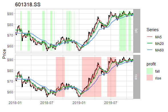
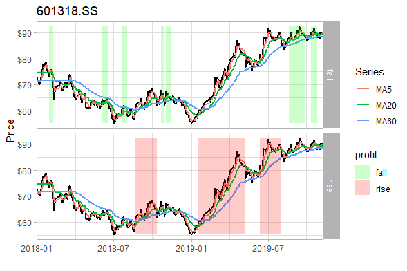
Suppose we set the buy filter as the slope of the 5-day average is greater than 0.5 (the inclination angle is about 26.5 °), that is to say, the slope of the 5-day average of the buy signal is greater than 0.5 to really buy. From January 1, 2018 to November 7, 2019 (the deadline of the last analysis), there are 20 transactions (total sales) and 6 profitable transactions. The final principal was 99788.09 and the loss was 211.91. The loss rate dropped from 19% to 0.02%. We can also see from the figure that the filter filters some transactions during the shock period.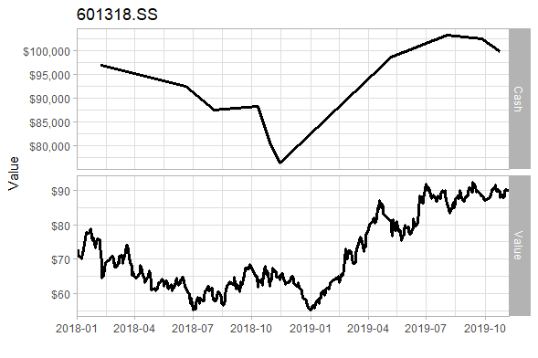

Questions

These methods can help us avoid trading in the period of shock to a certain extent, but if we want to use these methods exactly, then how many specific numbers should be set to be appropriate, that is, how many days should a stock be delayed to avoid the period of shock? Or how many stop loss lines? Or how much is the slope of the mean line set for filtering? In the future, I have the chance to play with some more advanced methods.

Related articles:
R and money game: golden cross 1