GTSAM Tutorial learning notes
In order to learn LIO-SAM, I quickly read Robot Perception: application of factor graph in SLAM and GTSAM Tutorial shared by big brother Dong Jing in bubble robot. The content of this blog is mainly the learning notes of GTSAM Tutorial, and make some simple analysis on the practical application of GTSAM in LIO-SAM, If you have a basic understanding of GTSAM, you can skip to the third part directly.
1. Basic principles
The following figure shows a typical SLAM scenario
The observation of feature points by the robot can be constructed as a Bayesian network as shown in the left figure above
x
i
x_i
xi is in robot state,
z
i
z_i
zi is the robot observation value,
l
i
l_i
li is the feature point. The joint distribution probability of such a Bayesian network can be expressed by the following formula:
P
(
X
,
L
,
Z
)
=
P
(
x
0
)
∏
i
=
1
M
P
(
x
i
∣
x
i
−
1
,
u
i
)
∏
k
=
1
K
P
(
z
k
∣
x
i
k
,
l
j
k
)
P(X, L, Z)=P\left(x_{0}\right) \prod_{i=1}^{M} P\left(x_{i} \mid x_{i-1}, u_{i}\right) \prod_{k=1}^{K} P\left(z_{k} \mid x_{i_{k}}, l_{j_{k}}\right)
P(X,L,Z)=P(x0) i=1 Π M P(xi ∣ xi − 1, ui) k=1 Π K P(zk ∣ xik, ljk), where,
P
(
x
0
)
P\left(x_{0}\right)
P(x0) is a priori state probability distribution,
P
(
x
i
∣
x
i
−
1
,
u
i
)
P\left(x_{i} \mid x_{i-1}, u_{i}\right)
P(xi ∣ xi − 1, ui) indicates a known state
x
i
−
1
x_{i-1}
xi − 1 − and control quantity
u
i
u_{i}
In the case of ui# distribution,
x
i
\boldsymbol{x}_{i}
xi , probability distribution, specifically:
x
i
=
f
i
(
x
i
−
1
,
u
i
)
+
w
i
⇔
x_{i}=f_{i}\left(x_{i-1}, u_{i}\right)+w_{i} \quad \Leftrightarrow
xi=fi(xi−1,ui)+wi⇔
P
(
x
i
∣
x
i
−
1
,
u
i
)
∝
exp
−
1
2
∥
f
i
(
x
i
−
1
,
u
i
)
−
x
i
∥
Λ
i
2
P\left(x_{i} \mid x_{i-1}, u_{i}\right) \propto \exp -\frac{1}{2}\left\|f_{i}\left(x_{i-1}, u_{i}\right)-x_{i}\right\|_{\Lambda_{i}}^{2}
P(xi∣xi−1,ui)∝exp−21∥fi(xi−1,ui)−xi∥Λi2
P
(
z
k
∣
x
i
k
,
l
j
k
)
P\left(z_{k} \mid x_{i_{k}}, l_{j_{k}}\right)
P(zk ∣ xik, ljk) indicates known status
x
i
k
\boldsymbol{x}_{i_{k}}
xik , and
l
j
k
l_{j_{k}}
In the case of ljk distribution,
z
k
z_{k}
The probability distribution of zk , is as follows:
z
k
=
h
k
(
x
i
k
,
l
j
k
)
+
v
k
⇔
z_{k}=h_{k}\left(x_{i_{k}}, l_{j_{k}}\right)+v_{k} \quad \Leftrightarrow
zk=hk(xik,ljk)+vk⇔
P
(
z
k
∣
x
i
k
,
l
j
k
)
∝
exp
−
1
2
∥
h
k
(
x
i
k
,
l
j
k
)
−
z
k
∥
Σ
k
2
P\left(z_{k} \mid x_{i_{k}}, l_{j_{k}}\right) \propto \exp -\frac{1}{2}\left\|h_{k}\left(x_{i_{k}}, l_{j_{k}}\right)-z_{k}\right\|_{\Sigma_{k}}^{2}
P(zk∣xik,ljk)∝exp−21∥hk(xik,ljk)−zk∥ Σ k ﹐ 2 ﹐ if the above distributions are assumed to be Gaussian, the following factor diagram can be constructed:
We express the above factor diagram by the following formula:
P
(
Θ
)
∝
∏
i
ϕ
i
(
θ
i
)
∏
{
i
,
j
}
,
i
<
j
ψ
i
j
(
θ
i
,
θ
j
)
,
Θ
≜
(
X
,
L
)
P(\Theta) \propto \prod_{i} \phi_{i}\left(\theta_{i}\right) \prod_{\{i, j\}, i<j} \psi_{i j}\left(\theta_{i}, \theta_{j}\right),\Theta \triangleq(X, L)
P( Θ) ∝i∏ ϕ i( θ i){i,j},i<j∏ ψ ij( θ i, θ j), Θ ≜ (X,L) where
ϕ
0
(
x
0
)
∝
P
(
x
0
)
\phi_{0}\left(x_{0}\right) \propto P\left(x_{0}\right)
ϕ0(x0)∝P(x0)
ψ
(
i
−
1
)
i
(
x
i
−
1
,
x
i
)
∝
P
(
x
i
∣
x
i
−
1
,
u
i
)
\psi_{(i-1) i}\left(x_{i-1}, x_{i}\right) \propto P\left(x_{i} \mid x_{i-1}, u_{i}\right)
ψ(i−1)i(xi−1,xi)∝P(xi∣xi−1,ui)
ψ
i
k
j
k
(
x
i
k
,
l
j
k
)
∝
P
(
z
k
∣
x
i
k
,
l
j
k
)
\psi_{i_{k} j_{k}}\left(x_{i_{k}}, l_{j_{k}}\right) \propto P\left(z_{k} \mid x_{i_{k}}, l_{j_{k}}\right)
ψ ik ∝ jk (xik, ljk) ∝ P(zk ∣ xik, ljk) in this way, we equivalent the robot state and the surrounding map points to a factor in the factor graph. In fact, the posterior probability of the whole factor graph can be modeled as the product of the posterior probability between all factors:
f
(
Θ
)
=
∏
i
f
i
(
Θ
i
)
Θ
≜
(
X
,
L
)
for each
f
i
(
Θ
i
)
∝
exp
(
−
1
2
∥
h
i
(
Θ
i
)
−
z
i
∥
Σ
i
2
)
f(\Theta)=\prod_{i} f_{i}\left(\Theta_{i}\right) \quad \Theta \triangleq(X, L) \quad \text { for each } f_{i}\left(\Theta_{i}\right) \propto \exp \left(-\frac{1}{2}\left\|h_{i}\left(\Theta_{i}\right)-z_{i}\right\|_{\Sigma_{i}}^{2}\right)
f( Θ)= i∏fi( Θ i) Θ ≜(X,L) for each fi( Θ i)∝exp(−21∥hi( Θ i)−zi∥ Σ I # 2) and our goal is to maximize the total a posteriori probability:
Θ
∗
increase
amount
excellent
turn
:
=
arg
max
Θ
f
(
Θ
)
\Theta ^ {* incremental Optimization:} = \ underset {\ theta} {\ Arg \ Max} f (\ theta)
Θ * incremental Optimization:= Θ argmaxf( Θ) The intuitive understanding is to solve what kind of robot state and map point distribution can maximize the probability of all current observations. Because it is a Gaussian probability distribution, we usually transfer the probability distribution to the logarithmic domain:
arg
min
Θ
(
−
log
f
(
Θ
)
)
=
arg
min
Θ
1
2
∑
i
∥
h
i
(
Θ
i
)
−
z
i
∥
Σ
i
2
\underset{\Theta}{\arg \min }(-\log f(\Theta))=\underset{\Theta}{\arg \min } \frac{1}{2} \sum_{i}\left\|h_{i}\left(\Theta_{i}\right)-z_{i}\right\|_{\Sigma_{i}}^{2}
Θ argmin(−logf( Θ))=Θ argmin21i∑∥hi( Θ i)−zi∥ Σ I # 2 # the solution of this problem is mainly through nonlinear optimization algorithms, such as Gauss Newton method or lewnberg method. The whole solution process is as follows
Here are a few points to note:
- Incremental Optimization: the above description is about the solution of a fixed Batch data, while the actual SLAM problem is an incremental problem. In the method of incremental optimization based on back-end optimization, the sliding window is usually used to optimize the local map, while in GTSAM, the incremental optimization is realized through the Bayers Tree built by iSAM2, as shown in the following figure, the red area table Shows the area optimized by GTSAM. GTSAM will only take the state and map points close to the current state for optimization. Even if a loop is generated, it will only be optimized around the loop area. For details of this part, see iSAM2: Incremental Smoothing and Mapping Using the Bayes Tree.
- Automatic sorting: we know that whether in Gauss Newton method or lewnberg method, an important step is to solve A X = b AX=b AX=b, there are usually two methods to solve the matrix: QR decomposition and Cholesky decomposition, in which QR decomposition is as follows: Q T A = [ R 0 ] Q T b = [ d e ] Q^{T} A=\left[\begin{array}{l} R \\ 0 \end{array}\right] \quad Q^{T} b=\left[\begin{array}{l} d \\ e \end{array}\right] QTA=[R0]QTb=[de] R δ = d R \delta=d R δ= dCholesky is decomposed as follows: A T A δ ∗ = A T b A^{T} A \delta^{*}=A^{T} b ATAδ∗=ATb I ≜ A T A = R T R \mathcal{I} \triangleq A^{T} A=R^{T} R I≜ATA=RTR first R T y = A T b and then R δ ∗ = y \text { first } R^{T} y=A^{T} b \text { and then } R \delta^{*}=y first RTy=ATb and then R δ * = the efficiency of Y Cholesky decomposition is one order of magnitude higher than QR decomposition in some cases, but the stability of Cholesky decomposition is not as good as QR decomposition when the matrix is approximately singular. However, no matter which decomposition method, the decomposition efficiency depends largely on the sparsity of the matrix. In GTSAM, we make our A matrix as sparse as possible through COLAMD algorithm, so as to improve the calculation efficiency.
2. Demo code
Provided in GTSAM Tutorial Demo code It describes how to construct a factor graph with loop as shown in the figure below
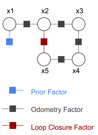
First, build a factor graph container
  // Create a factor graph container
  NonlinearFactorGraph graph;
Next, construct and add a priori factor, that is, the blue factor in the figure. Note that the factor is a unary edge
  // prior measurment noise model
  noiseModel::Diagonal::shared_ptr priorModel = noiseModel::Diagonal::Sigmas(Vector3(1.0, 1.0, 0.1));

  // Add a prior on the first pose, setting it to the origin
  // The prior is needed to fix/align the whole trajectory at world frame
  // A prior factor consists of a mean value and a noise model (covariance matrix)
  graph.add(PriorFactor<Pose2>(Symbol('x', 1), Pose2(0, 0, 0), priorModel));
Then construct and add odometer factors, that is, the black factors in the figure, which are binary edges
  // odometry measurement noise model (covariance matrix)
  noiseModel::Diagonal::shared_ptr odomModel = noiseModel::Diagonal::Sigmas(Vector3(0.5, 0.5, 0.1));

  // Add odometry factors
  // Create odometry (Between) factors between consecutive poses
  // robot makes 90 deg right turns at x3 - x5
  graph.add(BetweenFactor<Pose2>(Symbol('x', 1), Symbol('x', 2), Pose2(5, 0, 0), odomModel));
  graph.add(BetweenFactor<Pose2>(Symbol('x', 2), Symbol('x', 3), Pose2(5, 0, -M_PI_2), odomModel));
  graph.add(BetweenFactor<Pose2>(Symbol('x', 3), Symbol('x', 4), Pose2(5, 0, -M_PI_2), odomModel));
  graph.add(BetweenFactor<Pose2>(Symbol('x', 4), Symbol('x', 5), Pose2(5, 0, -M_PI_2), odomModel));
There is also the loop factor, that is, the red factor on the way, which is a binary edge
  // loop closure measurement noise model
  noiseModel::Diagonal::shared_ptr loopModel = noiseModel::Diagonal::Sigmas(Vector3(0.5, 0.5, 0.1));

  // Add the loop closure constraint
  graph.add(BetweenFactor<Pose2>(Symbol('x', 5), Symbol('x', 2), Pose2(5, 0, -M_PI_2), loopModel));
As can be seen from the above, the process of adding factors is to construct the noise model first, then add the factor type, the node connected by the factor and the initial value to the container of the factor graph, and then initialize the noise model of each node
  // initial varible values for the optimization
  // add random noise from ground truth values
  Values initials;
  initials.insert(Symbol('x', 1), Pose2(0.2, -0.3, 0.2));
  initials.insert(Symbol('x', 2), Pose2(5.1, 0.3, -0.1));
  initials.insert(Symbol('x', 3), Pose2(9.9, -0.1, -M_PI_2 - 0.2));
  initials.insert(Symbol('x', 4), Pose2(10.2, -5.0, -M_PI + 0.1));
  initials.insert(Symbol('x', 5), Pose2(5.1, -5.1, M_PI_2 - 0.1));
Finally, build the optimizer and perform optimization
  // Use Gauss-Newton method optimizes the initial values
  GaussNewtonParams parameters;

  // print per iteration
  parameters.setVerbosity("ERROR");

  // optimize!
  GaussNewtonOptimizer optimizer(graph, initials, parameters);
  Values results = optimizer.optimize();
The optimized residual value of each node can be obtained through the margins class
  // Calculate marginal covariances for all poses
  Marginals marginals(graph, results);

  // print marginal covariances
  cout << "x1 covariance:\n" << marginals.marginalCovariance(Symbol('x', 1)) << endl;
  cout << "x2 covariance:\n" << marginals.marginalCovariance(Symbol('x', 2)) << endl;
  cout << "x3 covariance:\n" << marginals.marginalCovariance(Symbol('x', 3)) << endl;
  cout << "x4 covariance:\n" << marginals.marginalCovariance(Symbol('x', 4)) << endl;
  cout << "x5 covariance:\n" << marginals.marginalCovariance(Symbol('x', 5)) << endl;
The above is the core part of the Demo code. It can be seen that the process of building factor graph by GTSAM is very simple and clear. Next, let's see how GTSAM is applied in practical projects.
3. Partial code analysis in lio-sam
The factor diagram constructed in LIO-SAM is as follows:
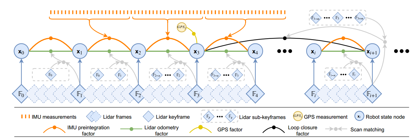
The above figure looks like a factor graph, but there are actually two types of factor graphs in LIO-SAM. the first factor graph is to build a factor graph with laser odometer and IMU pre product component between two laser odometers in imuintegration.cpp file to optimize the state of the current frame (including pose, speed and offset) Here, we call it pre integration factor graph. The second factor graph is to add factor graph to key frames in mapOptimization.cpp file, add laser odometer factor, GPS factor and closed-loop factor, perform factor graph optimization, and update the position and attitude of all key frames. Here, we call it key frame factor graph. Let's see the details below (refer to some code comments) LIO-SAM source code analysis):
3.1 pre integration factor diagram
The codes related to the pre integration factor graph are mainly in the IMUPreintegration class of imuintegration.cpp, which is defined as follows:
class IMUPreintegration : public ParamServer
{
public:
    std::mutex mtx;

	// Subscribe and Publish
	ros::Subscriber subImu;
	ros::Subscriber subOdometry;
	ros::Publisher pubImuOdometry;

	bool systemInitialized = false;

	// Noise covariance
	gtsam::noiseModel::Diagonal::shared_ptr priorPoseNoise;
	gtsam::noiseModel::Diagonal::shared_ptr priorVelNoise;
	gtsam::noiseModel::Diagonal::shared_ptr priorBiasNoise;
	gtsam::noiseModel::Diagonal::shared_ptr correctionNoise;
	gtsam::noiseModel::Diagonal::shared_ptr correctionNoise2;
	gtsam::Vector noiseModelBetweenBias;

	// imu pre integrator
	gtsam::PreintegratedImuMeasurements *imuIntegratorOpt_;
	gtsam::PreintegratedImuMeasurements *imuIntegratorImu_;

	// imu data queue
	std::deque<sensor_msgs::Imu> imuQueOpt;
	std::deque<sensor_msgs::Imu> imuQueImu;

	// State variables in imu factor graph optimization
	gtsam::Pose3 prevPose_;
	gtsam::Vector3 prevVel_;
	gtsam::NavState prevState_;
	gtsam::imuBias::ConstantBias prevBias_;

	// imu status
	gtsam::NavState prevStateOdom;
	gtsam::imuBias::ConstantBias prevBiasOdom;

	bool doneFirstOpt = false;
	double lastImuT_imu = -1;
	double lastImuT_opt = -1;

	// ISAM2 optimizer
	gtsam::ISAM2 optimizer;
	gtsam::NonlinearFactorGraph graphFactors;
	gtsam::Values graphValues;

	const double delta_t = 0;

	// Used to record the number of keyframes
	int key = 1;

	// IMU lidar pose transformation
	gtsam::Pose3 imu2Lidar = gtsam::Pose3(gtsam::Rot3(1, 0, 0, 0), gtsam::Point3(-extTrans.x(), -extTrans.y(), -extTrans.z()));
	gtsam::Pose3 lidar2Imu = gtsam::Pose3(gtsam::Rot3(1, 0, 0, 0), gtsam::Point3(extTrans.x(), extTrans.y(), extTrans.z()));

	// Constructor
    IMUPreintegration();

	// Reset iSAM2 optimizer
    void resetOptimization();

	// reset parameters
    void resetParams();

	// Subscription laser odometer
    void odometryHandler(const nav_msgs::Odometry::ConstPtr& odomMsg);

	// Determination of IMU factor graph optimization results
    bool failureDetection(const gtsam::Vector3& velCur, const gtsam::imuBias::ConstantBias& biasCur);

	// Subscribe to raw IMU data
    void imuHandler(const sensor_msgs::Imu::ConstPtr& imu_raw);
};
The member variables of the class include each state to be optimized and the noise covariance of each a priori factor. These parameters are initialized in the constructor. Let's see the contents of the constructor below:
IMUPreintegration()
{
    // Subscribe to the original imu data, apply the imu prediction component between two frames with the optimization result of the following factor diagram, and predict the imu odometer at each time (imu frequency)
    subImu      = nh.subscribe<sensor_msgs::Imu>  (imuTopic,                   2000, &IMUPreintegration::imuHandler,      this, ros::TransportHints().tcpNoDelay());
    // Subscribe to the laser odometer from mapOptimization, use the estimated imu component between two frames to build a factor map, and optimize the pose of the current frame (this pose is only used to update the imu odometer at each time and the next factor map optimization)
    subOdometry = nh.subscribe<nav_msgs::Odometry>("lio_sam/mapping/odometry_incremental", 5,    &IMUPreintegration::odometryHandler, this, ros::TransportHints().tcpNoDelay());

    // Issue imu odometer
    pubImuOdometry = nh.advertise<nav_msgs::Odometry> (odomTopic+"_incremental", 2000);

    // Noise covariance of imu pre integration
    boost::shared_ptr<gtsam::PreintegrationParams> p = gtsam::PreintegrationParams::MakeSharedU(imuGravity);
    p->accelerometerCovariance  = gtsam::Matrix33::Identity(3,3) * pow(imuAccNoise, 2); // acc white noise in continuous
    p->gyroscopeCovariance      = gtsam::Matrix33::Identity(3,3) * pow(imuGyrNoise, 2); // gyro white noise in continuous
    p->integrationCovariance    = gtsam::Matrix33::Identity(3,3) * pow(1e-4, 2); // error committed in integrating position from velocities
    gtsam::imuBias::ConstantBias prior_imu_bias((gtsam::Vector(6) << 0, 0, 0, 0, 0, 0).finished());; // assume zero initial bias

    // Noise a priori
    priorPoseNoise  = gtsam::noiseModel::Diagonal::Sigmas((gtsam::Vector(6) << 1e-2, 1e-2, 1e-2, 1e-2, 1e-2, 1e-2).finished()); // rad,rad,rad,m, m, m
    priorVelNoise   = gtsam::noiseModel::Isotropic::Sigma(3, 1e4); // m/s
    priorBiasNoise  = gtsam::noiseModel::Isotropic::Sigma(6, 1e-3); // 1e-2 ~ 1e-3 seems to be good
    // If the laser odometer degrades in the process of scan to map optimization, a large covariance is selected
    correctionNoise = gtsam::noiseModel::Diagonal::Sigmas((gtsam::Vector(6) << 0.05, 0.05, 0.05, 0.1, 0.1, 0.1).finished()); // rad,rad,rad,m, m, m
    correctionNoise2 = gtsam::noiseModel::Diagonal::Sigmas((gtsam::Vector(6) << 1, 1, 1, 1, 1, 1).finished()); // rad,rad,rad,m, m, m
    noiseModelBetweenBias = (gtsam::Vector(6) << imuAccBiasN, imuAccBiasN, imuAccBiasN, imuGyrBiasN, imuGyrBiasN, imuGyrBiasN).finished();

    // imu pre integrator, used to predict imu odometer at each time (imu frequency) (switch to lidar system, the same system as laser odometer)
    imuIntegratorImu_ = new gtsam::PreintegratedImuMeasurements(p, prior_imu_bias); // setting up the IMU integration for IMU message thread
    // imu pre integrator for factor graph optimization
    imuIntegratorOpt_ = new gtsam::PreintegratedImuMeasurements(p, prior_imu_bias); // setting up the IMU integration for optimization
}
Next, the core part of constructing the factor graph is in the subscription laser odometer function, as follows:
/**
 * Subscribe to laser odometer from mapOptimization
 * 1,Reset the ISAM2 optimizer every 100 frames, add odometer, speed and bias a priori factors, and perform optimization
 * 2,Calculate the imu pre product component between the previous frame laser odometer and the current frame laser odometer, apply the pre product component with the previous frame state to obtain the initial state estimation of the current frame, add the current frame pose from mapOptimization, optimize the factor graph and update the current frame state
 * 3,After optimization, re propagation is performed; The imu offset is optimized and updated. The imu pre integration after the current laser odometer time is recalculated with the latest offset. This pre integration is used to calculate the pose at each time
*/
void odometryHandler(const nav_msgs::Odometry::ConstPtr& odomMsg)
{
    std::lock_guard<std::mutex> lock(mtx);
    // Time stamp of laser odometer in current frame
    double currentCorrectionTime = ROS_TIME(odomMsg);

    // Ensure that there is imu data in the imu optimization queue for pre integration
    if (imuQueOpt.empty())
        return;

    // The laser pose of the current frame comes from the pose after scan to map matching and factor map optimization
    float p_x = odomMsg->pose.pose.position.x;
    float p_y = odomMsg->pose.pose.position.y;
    float p_z = odomMsg->pose.pose.position.z;
    float r_x = odomMsg->pose.pose.orientation.x;
    float r_y = odomMsg->pose.pose.orientation.y;
    float r_z = odomMsg->pose.pose.orientation.z;
    float r_w = odomMsg->pose.pose.orientation.w;
    bool degenerate = (int)odomMsg->pose.covariance[0] == 1 ? true : false;
    gtsam::Pose3 lidarPose = gtsam::Pose3(gtsam::Rot3::Quaternion(r_w, r_x, r_y, r_z), gtsam::Point3(p_x, p_y, p_z));


    // 0. System initialization, first frame
    if (systemInitialized == false)
    {
        // Reset ISAM2 optimizer
        resetOptimization();

        // Delete the imu data before the laser odometer time of the current frame from the imu optimization queue
        while (!imuQueOpt.empty())
        {
            if (ROS_TIME(&imuQueOpt.front()) < currentCorrectionTime - delta_t)
            {
                lastImuT_opt = ROS_TIME(&imuQueOpt.front());
                imuQueOpt.pop_front();
            }
            else
                break;
        }
        // Add odometer pose prior factor
        prevPose_ = lidarPose.compose(lidar2Imu);
        gtsam::PriorFactor<gtsam::Pose3> priorPose(X(0), prevPose_, priorPoseNoise);
        graphFactors.add(priorPose);
        // Add speed a priori factor
        prevVel_ = gtsam::Vector3(0, 0, 0);
        gtsam::PriorFactor<gtsam::Vector3> priorVel(V(0), prevVel_, priorVelNoise);
        graphFactors.add(priorVel);
        // Add imu bias a priori factor
        prevBias_ = gtsam::imuBias::ConstantBias();
        gtsam::PriorFactor<gtsam::imuBias::ConstantBias> priorBias(B(0), prevBias_, priorBiasNoise);
        graphFactors.add(priorBias);
        // Initial value of variable node
        graphValues.insert(X(0), prevPose_);
        graphValues.insert(V(0), prevVel_);
        graphValues.insert(B(0), prevBias_);
        // Optimize once
        optimizer.update(graphFactors, graphValues);
        graphFactors.resize(0);
        graphValues.clear();

        // Reset optimized offset
        imuIntegratorImu_->resetIntegrationAndSetBias(prevBias_);
        imuIntegratorOpt_->resetIntegrationAndSetBias(prevBias_);

        key = 1;
        systemInitialized = true;
        return;
    }


    // Reset the ISAM2 optimizer every 100 frames to ensure the optimization efficiency
    if (key == 100)
    {
        // Pose, velocity and bias noise model of the previous frame
        gtsam::noiseModel::Gaussian::shared_ptr updatedPoseNoise = gtsam::noiseModel::Gaussian::Covariance(optimizer.marginalCovariance(X(key-1)));
        gtsam::noiseModel::Gaussian::shared_ptr updatedVelNoise  = gtsam::noiseModel::Gaussian::Covariance(optimizer.marginalCovariance(V(key-1)));
        gtsam::noiseModel::Gaussian::shared_ptr updatedBiasNoise = gtsam::noiseModel::Gaussian::Covariance(optimizer.marginalCovariance(B(key-1)));
        // Reset ISAM2 optimizer
        resetOptimization();
        // Add pose a priori factor and initialize with the value of the previous frame
        gtsam::PriorFactor<gtsam::Pose3> priorPose(X(0), prevPose_, updatedPoseNoise);
        graphFactors.add(priorPose);
        // Add a speed a priori factor and initialize with the value of the previous frame
        gtsam::PriorFactor<gtsam::Vector3> priorVel(V(0), prevVel_, updatedVelNoise);
        graphFactors.add(priorVel);
        // Add an offset a priori factor and initialize with the value of the previous frame
        gtsam::PriorFactor<gtsam::imuBias::ConstantBias> priorBias(B(0), prevBias_, updatedBiasNoise);
        graphFactors.add(priorBias);
        // The variable node is assigned an initial value and initialized with the value of the previous frame
        graphValues.insert(X(0), prevPose_);
        graphValues.insert(V(0), prevVel_);
        graphValues.insert(B(0), prevBias_);
        // Optimize once
        optimizer.update(graphFactors, graphValues);
        graphFactors.resize(0);
        graphValues.clear();

        key = 1;
    }


    // 1. Calculate the imu pre product component between the previous frame and the current frame, apply the pre product component with the previous frame state to obtain the initial state estimation of the current frame, add the current frame pose from mapOptimization, optimize the factor graph and update the current frame state
    while (!imuQueOpt.empty())
    {
        // Extract the imu data between the previous frame and the current frame and calculate the pre integration
        sensor_msgs::Imu *thisImu = &imuQueOpt.front();
        double imuTime = ROS_TIME(thisImu);
        if (imuTime < currentCorrectionTime - delta_t)
        {
            // Time interval between two frames of imu data
            double dt = (lastImuT_opt < 0) ? (1.0 / 500.0) : (imuTime - lastImuT_opt);
            // imu pre integration data input: acceleration, angular velocity, dt
            imuIntegratorOpt_->integrateMeasurement(
                    gtsam::Vector3(thisImu->linear_acceleration.x, thisImu->linear_acceleration.y, thisImu->linear_acceleration.z),
                    gtsam::Vector3(thisImu->angular_velocity.x,    thisImu->angular_velocity.y,    thisImu->angular_velocity.z), dt);

            lastImuT_opt = imuTime;
            // Delete the processed imu data from the queue
            imuQueOpt.pop_front();
        }
        else
            break;
    }
    // Add imu pre integration factor
    const gtsam::PreintegratedImuMeasurements& preint_imu = dynamic_cast<const gtsam::PreintegratedImuMeasurements&>(*imuIntegratorOpt_);
    // Parameters: pose of previous frame, velocity of previous frame, pose of current frame, velocity of current frame, offset of previous frame, pre product component
    gtsam::ImuFactor imu_factor(X(key - 1), V(key - 1), X(key), V(key), B(key - 1), preint_imu);
    graphFactors.add(imu_factor);
    // Add imu offset factor, previous frame offset, current frame offset, observation value and noise covariance; deltaTij() is the time of the integration section
    graphFactors.add(gtsam::BetweenFactor<gtsam::imuBias::ConstantBias>(B(key - 1), B(key), gtsam::imuBias::ConstantBias(),
                        gtsam::noiseModel::Diagonal::Sigmas(sqrt(imuIntegratorOpt_->deltaTij()) * noiseModelBetweenBias)));
    // Add pose factor
    gtsam::Pose3 curPose = lidarPose.compose(lidar2Imu);
    gtsam::PriorFactor<gtsam::Pose3> pose_factor(X(key), curPose, degenerate ? correctionNoise2 : correctionNoise);
    graphFactors.add(pose_factor);
    // Using the state and offset of the previous frame, the imu prediction component is applied to obtain the state of the current frame
    gtsam::NavState propState_ = imuIntegratorOpt_->predict(prevState_, prevBias_);
    // Initial value of variable node
    graphValues.insert(X(key), propState_.pose());
    graphValues.insert(V(key), propState_.v());
    graphValues.insert(B(key), prevBias_);
    // optimization
    optimizer.update(graphFactors, graphValues);
    optimizer.update();
    graphFactors.resize(0);
    graphValues.clear();
    // Optimization results
    gtsam::Values result = optimizer.calculateEstimate();
    // Update the pose and speed of the current frame
    prevPose_  = result.at<gtsam::Pose3>(X(key));
    prevVel_   = result.at<gtsam::Vector3>(V(key));
    // Update current frame status
    prevState_ = gtsam::NavState(prevPose_, prevVel_);
    // Update current frame imu offset
    prevBias_  = result.at<gtsam::imuBias::ConstantBias>(B(key));
    // Reset the pre integrator and set a new offset, so that when the laser odometer comes in the next frame, the pre integrator component is the increment between two frames
    imuIntegratorOpt_->resetIntegrationAndSetBias(prevBias_);

    // If the speed or offset of imu factor graph optimization result is too large, it is considered as failure
    if (failureDetection(prevVel_, prevBias_))
    {
        // reset parameters
        resetParams();
        return;
    }


    // 2. After optimization, perform re propagation; The imu offset is optimized and updated. The imu pre integration after the current laser odometer time is recalculated with the latest offset. This pre integration is used to calculate the pose at each time
    prevStateOdom = prevState_;
    prevBiasOdom  = prevBias_;
    // Delete the imu data before the current laser odometer time from the imu queue
    double lastImuQT = -1;
    while (!imuQueImu.empty() && ROS_TIME(&imuQueImu.front()) < currentCorrectionTime - delta_t)
    {
        lastImuQT = ROS_TIME(&imuQueImu.front());
        imuQueImu.pop_front();
    }
    // Pre integration is calculated for the remaining imu data
    if (!imuQueImu.empty())
    {
        // Reset the pre integrator and the latest offset
        imuIntegratorImu_->resetIntegrationAndSetBias(prevBiasOdom);
        // Calculate pre integration
        for (int i = 0; i < (int)imuQueImu.size(); ++i)
        {
            sensor_msgs::Imu *thisImu = &imuQueImu[i];
            double imuTime = ROS_TIME(thisImu);
            double dt = (lastImuQT < 0) ? (1.0 / 500.0) :(imuTime - lastImuQT);

            imuIntegratorImu_->integrateMeasurement(gtsam::Vector3(thisImu->linear_acceleration.x, thisImu->linear_acceleration.y, thisImu->linear_acceleration.z),
                                                    gtsam::Vector3(thisImu->angular_velocity.x,    thisImu->angular_velocity.y,    thisImu->angular_velocity.z), dt);
            lastImuQT = imuTime;
        }
    }

    ++key;
    doneFirstOpt = true;
}
One of the more special points is the use of the gtsam::PreintegratedImuMeasurements class. Finding a class is equivalent to encapsulating a pile of preintegrations and their Jacobian derivation formulas. It's not too cool. We can also see from the code that the slightly more complex part in the process of building factor graph is the given process of Noise Model of factor.
3.2 key frame factor diagram
The codes related to the key frame factor graph are mainly in the savekeyframeandfactor function of mapOptimization.cpp. In mapOptimization.cpp, in addition to the key frame factor graph, it also includes the matching algorithm of scan to map, key frame determination, etc. we will not introduce these codes too much. The savekeyframeandfactor function is as follows:
/**
 * Set the current frame as a key frame and perform factor graph optimization
 * 1,Calculate the pose transformation between the current frame and the previous frame. If the change is too small, it will not be set as a key frame, otherwise it will be set as a key frame
 * 2,Add laser odometer factor, GPS factor and closed-loop factor
 * 3,Execution factor graph optimization
 * 4,The optimized pose and pose covariance of the current frame are obtained
 * 5,Add cloudKeyPoses3D and cloudKeyPoses6D, update transformTobeMapped, and add the corner and plane point collection of the current key frame
*/
void saveKeyFramesAndFactor()
{
    // Calculate the pose transformation between the current frame and the previous frame. If the change is too small, it will not be set as a key frame, otherwise it will be set as a key frame
    if (saveFrame() == false)
        return;

    // Laser odometer factor
    addOdomFactor();

    // GPS factor
    addGPSFactor();

    // Closed loop factor
    addLoopFactor();

    // cout << "****************************************************" << endl;
    // gtSAMgraph.print("GTSAM Graph:\n");

    // Execution optimization
    isam->update(gtSAMgraph, initialEstimate);
    isam->update();

    if (aLoopIsClosed == true)
    {
        isam->update();
        isam->update();
        isam->update();
        isam->update();
        isam->update();
    }

    // After update, clear the saved factor graph. Note: the historical data will not be cleared, but the ISAM will be saved
    gtSAMgraph.resize(0);
    initialEstimate.clear();

    PointType thisPose3D;
    PointTypePose thisPose6D;
    Pose3 latestEstimate;

    // Optimization results
    isamCurrentEstimate = isam->calculateEstimate();
    // Pose result of current frame
    latestEstimate = isamCurrentEstimate.at<Pose3>(isamCurrentEstimate.size()-1);
    // cout << "****************************************************" << endl;
    // isamCurrentEstimate.print("Current estimate: ");

    // cloudKeyPoses3D adds the pose of the current frame
    thisPose3D.x = latestEstimate.translation().x();
    thisPose3D.y = latestEstimate.translation().y();
    thisPose3D.z = latestEstimate.translation().z();
    // Indexes
    thisPose3D.intensity = cloudKeyPoses3D->size();
    cloudKeyPoses3D->push_back(thisPose3D);

    // Cloudkeypose6d adds the pose of the current frame
    thisPose6D.x = thisPose3D.x;
    thisPose6D.y = thisPose3D.y;
    thisPose6D.z = thisPose3D.z;
    thisPose6D.intensity = thisPose3D.intensity ;
    thisPose6D.roll  = latestEstimate.rotation().roll();
    thisPose6D.pitch = latestEstimate.rotation().pitch();
    thisPose6D.yaw   = latestEstimate.rotation().yaw();
    thisPose6D.time = timeLaserInfoCur;
    cloudKeyPoses6D->push_back(thisPose6D);

    // cout << "****************************************************" << endl;
    // cout << "Pose covariance:" << endl;
    // cout << isam->marginalCovariance(isamCurrentEstimate.size()-1) << endl << endl;
    // Pose covariance
    poseCovariance = isam->marginalCovariance(isamCurrentEstimate.size()-1);

    // transformTobeMapped updates the pose of the current frame
    transformTobeMapped[0] = latestEstimate.rotation().roll();
    transformTobeMapped[1] = latestEstimate.rotation().pitch();
    transformTobeMapped[2] = latestEstimate.rotation().yaw();
    transformTobeMapped[3] = latestEstimate.translation().x();
    transformTobeMapped[4] = latestEstimate.translation().y();
    transformTobeMapped[5] = latestEstimate.translation().z();

    // Current frame laser corner, plane point, downsampling set
    pcl::PointCloud<PointType>::Ptr thisCornerKeyFrame(new pcl::PointCloud<PointType>());
    pcl::PointCloud<PointType>::Ptr thisSurfKeyFrame(new pcl::PointCloud<PointType>());
    pcl::copyPointCloud(*laserCloudCornerLastDS,  *thisCornerKeyFrame);
    pcl::copyPointCloud(*laserCloudSurfLastDS,    *thisSurfKeyFrame);

    // Save feature point downsampling set
    cornerCloudKeyFrames.push_back(thisCornerKeyFrame);
    surfCloudKeyFrames.push_back(thisSurfKeyFrame);

    // Update odometer track
    updatePath(thisPose6D);
}
The optimization results of all state variables in history are saved in isamCurrentEstimate, while the results of the latest frame are saved in latestEstimate, where the function of adding odometer factor is
void addOdomFactor()
{
    if (cloudKeyPoses3D->points.empty())
    {
        noiseModel::Diagonal::shared_ptr priorNoise = noiseModel::Diagonal::Variances((Vector(6) << 1e-2, 1e-2, M_PI*M_PI, 1e8, 1e8, 1e8).finished()); // rad*rad, meter*meter
        gtSAMgraph.add(PriorFactor<Pose3>(0, trans2gtsamPose(transformTobeMapped), priorNoise));
        initialEstimate.insert(0, trans2gtsamPose(transformTobeMapped));
    }else{
        noiseModel::Diagonal::shared_ptr odometryNoise = noiseModel::Diagonal::Variances((Vector(6) << 1e-6, 1e-6, 1e-6, 1e-4, 1e-4, 1e-4).finished());
        gtsam::Pose3 poseFrom = pclPointTogtsamPose3(cloudKeyPoses6D->points.back());
        gtsam::Pose3 poseTo   = trans2gtsamPose(transformTobeMapped);
        gtSAMgraph.add(BetweenFactor<Pose3>(cloudKeyPoses3D->size()-1, cloudKeyPoses3D->size(), poseFrom.between(poseTo), odometryNoise));
        initialEstimate.insert(cloudKeyPoses3D->size(), poseTo);
    }
}
Adding GPS factor function is relatively complex, so it is necessary to judge whether to add and interpolate:
void addGPSFactor()
{
    if (gpsQueue.empty())
        return;

    // wait for system initialized and settles down
    if (cloudKeyPoses3D->points.empty())
        return;
    else
    {
        if (pointDistance(cloudKeyPoses3D->front(), cloudKeyPoses3D->back()) < 5.0)
            return;
    }

    // pose covariance small, no need to correct
    if (poseCovariance(3,3) < poseCovThreshold && poseCovariance(4,4) < poseCovThreshold)
        return;

    // last gps position
    static PointType lastGPSPoint;

    while (!gpsQueue.empty())
    {
        if (gpsQueue.front().header.stamp.toSec() < timeLaserInfoCur - 0.2)
        {
            // message too old
            gpsQueue.pop_front();
        }
        else if (gpsQueue.front().header.stamp.toSec() > timeLaserInfoCur + 0.2)
        {
            // message too new
            break;
        }
        else
        {
            nav_msgs::Odometry thisGPS = gpsQueue.front();
            gpsQueue.pop_front();

            // GPS too noisy, skip
            float noise_x = thisGPS.pose.covariance[0];
            float noise_y = thisGPS.pose.covariance[7];
            float noise_z = thisGPS.pose.covariance[14];
            if (noise_x > gpsCovThreshold || noise_y > gpsCovThreshold)
                continue;

            float gps_x = thisGPS.pose.pose.position.x;
            float gps_y = thisGPS.pose.pose.position.y;
            float gps_z = thisGPS.pose.pose.position.z;
            if (!useGpsElevation)
            {
                gps_z = transformTobeMapped[5];
                noise_z = 0.01;
            }

            // GPS not properly initialized (0,0,0)
            if (abs(gps_x) < 1e-6 && abs(gps_y) < 1e-6)
                continue;

            // Add GPS every a few meters
            PointType curGPSPoint;
            curGPSPoint.x = gps_x;
            curGPSPoint.y = gps_y;
            curGPSPoint.z = gps_z;
            if (pointDistance(curGPSPoint, lastGPSPoint) < 5.0)
                continue;
            else
                lastGPSPoint = curGPSPoint;

            gtsam::Vector Vector3(3);
            Vector3 << max(noise_x, 1.0f), max(noise_y, 1.0f), max(noise_z, 1.0f);
            noiseModel::Diagonal::shared_ptr gps_noise = noiseModel::Diagonal::Variances(Vector3);
            gtsam::GPSFactor gps_factor(cloudKeyPoses3D->size(), gtsam::Point3(gps_x, gps_y, gps_z), gps_noise);
            gtSAMgraph.add(gps_factor);

            aLoopIsClosed = true;
            break;
        }
    }
}
Add the loopback factor function as follows:
void addLoopFactor()
{
    if (loopIndexQueue.empty())
        return;

    for (int i = 0; i < (int)loopIndexQueue.size(); ++i)
    {
        int indexFrom = loopIndexQueue[i].first;
        int indexTo = loopIndexQueue[i].second;
        gtsam::Pose3 poseBetween = loopPoseQueue[i];
        gtsam::noiseModel::Diagonal::shared_ptr noiseBetween = loopNoiseQueue[i];
        gtSAMgraph.add(BetweenFactor<Pose3>(indexFrom, indexTo, poseBetween, noiseBetween));
    }

    loopIndexQueue.clear();
    loopPoseQueue.clear();
    loopNoiseQueue.clear();
    aLoopIsClosed = true;
}
Then, the above briefly introduces the application of GTSAM in leo-sam project. The introduction is still rough. I will add it slowly later. I have just contacted GTSAM. If you have any questions, welcome to communicate!