A common step in data analysis is to group data sets and then apply functions, which can also be called grouping operations. The God Hadley Wickham coined the term split-apply-combine, which means split-application-merge. So when we talk about grouping operations, what are we actually talking about?

• Splitting: Dividing and grouping data according to standards
• Applying: Applying a function to each group
• Combining: Merging results into new data structures

The data storage format required by grouping operation is "long format", so the conversion of "long format" and "wide format" is introduced first, and then the specific operation of grouping operation.

"Long Format" VS "Wide Format“

There are two common ways to save data, long format or wide format.

• wide format

gene	meristem	root	FLOWER
gene1	582	91	495
gene2	305	3505	33

In a wide format, category variables are arranged separately. For example, the different parts of the plant above are divided into three columns, in which the data are expressed as the quantity of expression. It seems very intuitive, and it's the same way to record data in everyday life.

• long format

gene	organization	Expression quantity
gene1	meristem	582
gene2	meristem	305
gene1	root	91
gene2	root	3503
gene1	FLOWER	492
gene2	FLOWER	33

Long-structured data is defined as a special column of categorical variables. Typically, relational databases (such as MySQL) store data in long formats, because category rows (such as organizations) can increase or decrease with the increase or deletion of data in tables under a fixed architecture.

Subsequent grouping operations actually tend to save data in long format, so here we first introduce how pandas can convert between long format and wide format.

First, create a long-formatted data for testing by:

import pandas.util.testing as tm; tm.N = 3
def unpivot(frame):
    N, K = frame.shape
    data = {'value' : frame.values.ravel('F'),
            'variable' : np.asarray(frame.columns).repeat(N),
            'date' : np.tile(np.asarray(frame.index), K)}
    return pd.DataFrame(data, columns=['date', 'variable', 'value'])
ldata = unpivot(tm.makeTimeDataFrame())

Then the long format is changed into the wide format, which can be regarded as "rotating" the columns of data into rows.

# The first method: pivot
# pd.pivot(index, columns, values), corresponding index, category column and numerical column
pivoted = ldata.pivot('date','variable','value')
# The second method: unstack
## Hierarchical indexing with set_index
unstacked = ldata.set_index(['date','varibale']).unstack('variable')

If the wide format is changed into the long format, it can also be considered that the rows of data are "rotated" into columns.

# First restore unstacked data to a normal DataFrame
wdata = nstacked.reset_index()
wdata.columns = ['date','A','B','C','D']
# The first method: melt
pd.melt(wdata, id_vars=['date'])
# The second method: stack
# If the original data is not indexed, it needs to be rebuilt with set_index
wdata.set_index('date').stack()

GroupBy

The first step is to divide data sets into groups according to certain criteria, i.e. grouping keys. pandas provides grouby methods that can work according to grouping keys as follows:

• Numpy array, whose length is the same as the axis to be grouped
• The value of a column name in the DataFrame
• Dictionary or Series, which provides the corresponding relationship between the values on the axis to be grouped and the label - > group name
• According to multi-level axis index
• Python function for each label in an axis index or index

The following examples are given:
Form 1: According to the value of a column, it is generally a categorical value.

df = DataFrame({'A' : ['foo', 'bar', 'foo', 'bar',
                          'foo', 'bar', 'foo', 'foo'],
                  'B' : ['one', 'one', 'two', 'three',
                          'two', 'two', 'one', 'three'],
                   'C' : np.random.randn(8),
                   'D' : np.random.randn(8)})
# Split by column A
df.groupby('A')
# Split by columns A and B
df.groupby(['A','B'])

This results in a pandas.core.groupby.DataFrameGroupBy object object object, which does not perform substantive operations, but produces only intermediate information. You can view the size of each group after grouping.

df.groupby(['A','B']).size()

Form 2: According to the function, a function is defined below to split the column names according to whether they belong to vowels or not.

def get_letter_type(letter):
    if letter.lower() in 'aeiou':
        return 'vowel'
    else:
        return 'consonant'

grouped = df.groupby(get_letter_type, axis=1).

Form 3: According to hierarchical index. Unlike the R language data.frame, which has only one row or column name, pandas's DataFrame allows multiple hierarchical row or column names.

# Data for building multi-level index
arrays = [['bar', 'bar', 'baz', 'baz', 'foo', 'foo', 'qux', 'qux'],
           ['one', 'two', 'one', 'two', 'one', 'two', 'one', 'two']]
index = pd.MultiIndex.from_arrays(arrays, names=['first', 'second'])
s = pd.Series(np.random.randn(8), index=index)
# Grouping according to different levels of index
level1 = s.groupby(level='first') # First floor
level2 = s.groupby(level=1) # The second floor

Form 4: Grouping by dictionary or Series
The mapping of grouping information can be defined by a dictionary.

mapping = {'A':'str','B':'str','C':'values','D':'values','E':'values'}
df.groupby(mapping, axis=1)

Form 4: Grouping by row index and column value at the same time

df.index = index
df.groupby([pd.Grouper(level='first'),'A']).mean()

Group Object Iteration: GroupBy grouping objects generated above can be iterated, resulting in a set of binary tuples.

# For single-key values
for name, group in df.groupby(['A']):
    print(name)
    print(group)
# For multiple key values
for (k1,k2), group in df.groupby(['A']):
    print(k1,k2)
    print(group)

Select Groups: We can extract a specific group with get_group() after the grouping is finished.

df.groupby('A').get_group('foo')
# Here are the results
                A      B         C         D         E
first second                                          
bar   one     foo    one  0.709603 -1.023657 -0.321730
baz   one     foo    two  1.495328 -0.279928 -0.297983
foo   one     foo    two  0.495288 -0.563845 -1.774453
qux   one     foo    one  1.649135 -0.274208  1.194536
      two     foo  three -2.194127  3.440418 -0.023144
# Multiple groups
df.groupby(['A', 'B']).get_group(('bar', 'one'))

Apply

The grouping step is more direct, while the application function step changes more. In this step, we may do the following:

• Aggregation: Calculate the statistical information of each group separately, such as mean, size, etc.
• Transformation s: Specific calculations for each group, such as standardization, missing interpolation, etc.
• Filtration: Screening based on statistical information, discarding some groups.

Data aggregation: Aggregation

The so-called aggregation is the data conversion process in which arrays generate scalar values. We can use general methods such as mean, count, min, sum, etc. or aggregate or equivalent agg methods created by GroupBy objects.

grouped = df.groupby('A')
grouped.mean()
# Equivalent to
grouped.agg(np.mean)

For multiple groupings, the result of hierarchical indexing is generated. If you want the hierarchical indexing to be a separate column, you need to use the as_index option in groupby. Or finally use the reset_index method

# as_index
grouped = df.groupby(['A','B'], as_index=False)
grouped.agg(np.mean)
# reset_index
df.groupby(['A','B']).sum().reset_index()

aggregate or equivalent agg also allows multiple statistical functions for each column

df.groupby('A').agg([np.sum,np.mean,np.std])
# Grammatical sugar df.groupby('A').C is equivalent to
# grouped=df.groupby(['A'])
# grouped['C']
df.groupby('A').C.agg([np.sum,np.mean,np.std])

Or use different functions for different columns, such as calculating standard deviation for column D and averaging columns.

grouped=df.groupby(['A'])
grouped.agg({'D': np.std , 'C': np.mean})

Note: At present, the sum, mean, std and sem methods have been optimized for Cython.

Conversion: Transformation

The object returned by transform has the same size as the original grouped data. The functions used for conversion must satisfy the following conditions:

• Returns the same size as the original group chunk
• Column-by-column operation in block
• Not in-situ operations on blocks. The original block is considered immutable, and any modification to the original block may lead to unexpected results. If you use fillna, it must be grouped.transform(lambda x: x.fillna(inplace=False))

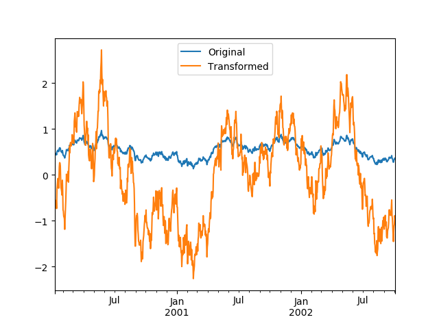
For example, we standardize each set of data. Of course, we have to first have a set of data, randomly generate a set from 1999 to 2002, and then take 100 days as a sliding window to calculate the mean value of each sliding window.

# date_range generates date index
index = pd.date_range('10/1/1999', periods=1100)
ts = pd.Series(np.random.normal(0.5, 2, 1100), index)
ts = ts.rolling(window=100,min_periods=100).mean().dropna()

Then, the data in each group should be standardized and zscore calculated by grouping according to the year.

# Two anonymous functions for grouping and calculating zscore
key = lambda x : x.year
zscore = lambda x : (x - x.mean())/x.std()
transformed = ts.groupby(key).transform(zscore)

broadcast technology is used in the application of zscore. Let's visualize the data shapes before and after the transformation

compare = pd.DataFrame({'Original': ts, 'Transformed': transformed})
compare.plot()

Filtering: Filtration

Filtering returns a subset of the original data. For example, the above time-Cycle data filters out years with an average value of less than 0.55.

ts.groupby(key).filter(lambda x : x.mean() > 0.55)

Apply: More Flexible "Split-App-Merge"

The aggregate and transform mentioned above have certain limitations. The function passed in can only produce two results, either a scalar value that can be broadcast or an array of the same size. apply is a more general function that can accomplish all the tasks described above and do better.

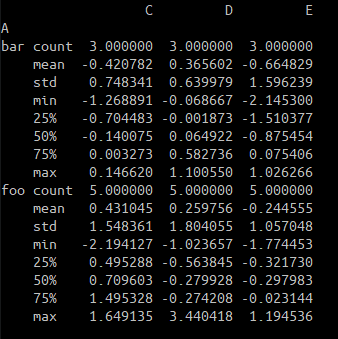
• Grouping returns descriptive statistics

df.groupby('A').apply(lambda x : x.describe())
# The effect is equivalent to df.groupby('A').describe()

• Modify the returned group name

def f(group):
     return pd.DataFrame({'original' : group,
                          'demeaned' : group - group.mean()})
df.groupby('A')['C'].apply(f)
              demeaned  original
first second                    
bar   one     0.278558  0.709603
      two     0.280707 -0.140075
baz   one     1.064283  1.495328
      two    -0.848109 -1.268891
foo   one     0.064243  0.495288
      two     0.567402  0.146620
qux   one     1.218089  1.649135
      two    -2.625172 -2.194127

For more useful tips, such as getting the nth line of each group, see Official documents