Wine quality data set
the wine quality data set includes two files - red wine file and white wine file. There are 1599 observations in the red wine file and 4898 observations in the white wine file. There are 1 output variable and 11 input variables in both files. The output variable is the quality of the wine, a score from 0 (low quality) to 10 (high quality). The input variables are the physical and chemical composition and characteristics of wine, including non-volatile acid, volatile acid, citric acid, residual sugar, chloride, free sulfur dioxide, total sulfur dioxide, density, pH value, sulfate and alcohol content.
. The dataset should include a header row and 6497 entries. In addition, another column should be added to distinguish whether this row of data is red wine or white wine.
Do you want to download the dataset? Point me!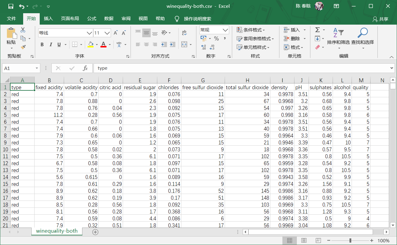
descriptive statistics
Let's analyze this dataset. First, we need to calculate the total descriptive statistics of each column, the unique value in the quality column and the number of observations corresponding to the unique value. The code is as follows:
#!/usr/bin/env python3

import numpy as np
import pandas as pd
import seaborn as sns
import matplotlib.pyplot as plt
import statsmodels.api as sm
import statsmodels.formula.api as smf
from statsmodels.formula.api import ols, glm

# Read the dataset into the pandas data box
wine = pd.read_csv('winequality-both.csv', sep=',', header=0)
wine.columns = wine.columns.str.replace(' ', '_')
print(wine.head())

# Show descriptive statistics for all variables
print(wine.describe())

# Find a unique value
print(sorted(wine.quality.unique()))

# Frequency of calculated value
print(wine.quality.value_counts())
after reading the text file into a pandas data box using the read csv() method of the pandas module, we use the head() function to check the header row and the first five rows of data to ensure that the data is loaded correctly. Line 17 uses pandas' description() function to print the summary statistics of each numeric variable in the dataset. Line 20 uses unique() to identify unique values in the quality column and print them on the screen in ascending order. Finally, line 23 calculates the number of times each unique value in the quality column appears in the dataset and prints them in descending order to the screen.
the running result of this code is as follows:
  type  fixed_acidity  volatile_acidity  ...  sulphates  alcohol  quality
0  red            7.4              0.70  ...       0.56      9.4        5
1  red            7.8              0.88  ...       0.68      9.8        5
2  red            7.8              0.76  ...       0.65      9.8        5
3  red           11.2              0.28  ...       0.58      9.8        6
4  red            7.4              0.70  ...       0.56      9.4        5

[5 rows x 13 columns]
       fixed_acidity  volatile_acidity  ...      alcohol      quality
count    6497.000000       6497.000000  ...  6497.000000  6497.000000
mean        7.215307          0.339666  ...    10.491801     5.818378
std         1.296434          0.164636  ...     1.192712     0.873255
min         3.800000          0.080000  ...     8.000000     3.000000
25%         6.400000          0.230000  ...     9.500000     5.000000
50%         7.000000          0.290000  ...    10.300000     6.000000
75%         7.700000          0.400000  ...    11.300000     6.000000
max        15.900000          1.580000  ...    14.900000     9.000000

[8 rows x 12 columns]
[3, 4, 5, 6, 7, 8, 9]
6    2836
5    2138
7    1079
4     216
8     193
3      30
9       5
Name: quality, dtype: int64
output shows that there are 6497 observations in the quality score, ranging from 3 to 9, with an average quality score of 5.8 and a standard deviation of 0.87; the only values in the quality column are 3, 4, 5, 6, 7, 8 and 9; the quality scores of 2836 observations are 62138 observations and 51079 observations and 7216 observations and 4193 observations The quality score of 30 observations is 3, and the quality score of 5 observations is 9.
Grouping, histogram and t-test
let's analyze the red wine data and white wine data respectively to see if the statistics will remain unchanged.
...
# Descriptive statistics showing quality by wine type
print(wine.groupby('type')[['quality']].describe().unstack('type'))
# Display quality specific quantile values by wine type
print(wine.groupby('type')[['quality']].quantile([0.25, 0.75]).unstack('type'))
# View quality distribution by wine type
red_wine = wine.loc[wine['type'] == 'red', 'quality']
white_wine = wine.loc[wine['type'] == 'white', 'quality']
sns.set_style("dark")
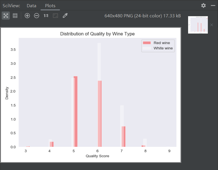
print(sns.distplot(red_wine, norm_hist=True, kde=False, color="red", label="Red wine"))
print(sns.distplot(white_wine, norm_hist=True, kde=False, color="white", label="White wine"))
sns.utils.axlabel("Quality Score", "Density")
plt.title("Distribution of Quality by Wine Type")
plt.legend()
plt.show()
# Check whether the average quality of red wine and white wine is different
print(wine.groupby(['type'])[['quality']].agg(['std']))
tstat, pvalue, df = sm.stats.ttest_ind(red_wine, white_wine)
print('tstat: %.3f pvalue: %.4f' % (tstat, pvalue))
The groupby() function uses two values in the type column to divide the data into two groups. Square brackets can generate a list of elements that are columns used to generate output. Here we apply the description () function only to the quality column. The result of these commands is to generate a list of statistics. The calculation results from red wine data and white wine data are stacked vertically with each other. The unstack() function rearranges the results so that red and white wine statistics are displayed in two columns side by side. The quantity() function evaluates the 25th and 75th percentiles of the mass column.
next, we use seaborn to create histograms, red bars for red wine and white bars for white wine. Because white wine has more data than red wine, histogram shows density distribution rather than frequency distribution.
. Here we want to know whether the standard deviation of red wine and white wine is the same, so we can use the combined variance in t test.
.
                type
quality  count  red      1599.000000
                white    4898.000000
         mean   red         5.636023
                white       5.877909
         std    red         0.807569
                white       0.885639
         min    red         3.000000
                white       3.000000
         25%    red         5.000000
                white       5.000000
         50%    red         6.000000
                white       6.000000
         75%    red         6.000000
                white       6.000000
         max    red         8.000000
                white       9.000000
dtype: float64
     quality
type     red white
0.25     5.0   5.0
0.75     6.0   6.0
AxesSubplot(0.125,0.11;0.775x0.77)
AxesSubplot(0.125,0.11;0.775x0.77)
        quality
            std
type
red    0.807569
white  0.885639
tstat: -9.686 pvalue: 0.0000
.
Relationship and correlation between paired variables
. Let's calculate the correlation between two input variables and create a scatter chart with regression lines for some input variables:
...
# Calculate the correlation matrix of all variables
print(wine.corr())
# Draw a "small" sample from red and white wine data
def take_sample(data_frame, replace=False, n=200):
return data_frame.loc[np.random.choice(data_frame.index, replace=replace, size=n)]
reds_sample = take_sample(wine.loc[wine['type'] == 'red', :])
whites_sample = take_sample(wine.loc[wine['type'] == 'white', :])
wine_sample = pd.concat([reds_sample, whites_sample])
wine['in_sample'] = np.where(wine.index.isin(wine_sample.index), 1., 0.)
print(pd.crosstab(wine.in_sample, wine.type, margins=True))
# View the relationship between pairs of variables
sns.set_style("dark")
g = sns.pairplot(wine_sample, kind='reg', plot_kws={"ci": False, "x_jitter": 0.25, "y_jitter": 0.25}, hue='type',
diag_kind='hist', diag_kws={"bins": 10, "alpha": 1.0}, palette=dict(red="red", white="white"),
markers=["o", "s"], vars=['quality', 'alcohol', 'residual_sugar'])
print(g)
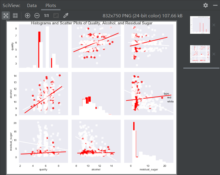
plt.suptitle('Histograms and Scatter Plots of Quality, Alcohol, and Residual Sugar', fontsize=14,
horizontalalignment='center', verticalalignment='top', x=0.5, y=0.999)
plt.show()
The corr() function calculates the linear correlation between the two variables in the dataset.
There are more than 6000 points in the dataset, so if they are all drawn in the statistical chart, it is difficult to distinguish the clear points. We define a function, take u sample(), to extract the sample points used in the statistical chart. This function uses the pandas data box index and numpy's random.choice() function to randomly select a subset of rows. We use this function to sample red wine and white wine respectively, and connect the two data frames obtained from sampling into one data frame. Then, create a new column in the wine data box, and use the where() function of numpy and the isin() function of pandas to fill in the new column. The filled value is set to 1 and 0 respectively according to whether the index value of this row is in the index value of sampling data. Finally, we use the crosstab() function of pandas to confirm that the IN'U sample column contains 400 1 (200 red wine data and 200 red wine data White wine data) and 6097 zeros.
The pairplot() function of seaborn can create a statistical graph matrix. The graph on the main diagonal shows the univariate distribution of each variable in the form of histogram or density graph. The graph outside the diagonal shows the bivariate distribution between each two variables in the form of scatter graph. The scatter graph can have regression line or not. Because the quality scores are all integers, adding a little vibration makes it easier to see where the data is concentrated.
the running result of this code is as follows:
                      fixed_acidity  volatile_acidity  ...   alcohol   quality
fixed_acidity              1.000000          0.219008  ... -0.095452 -0.076743
volatile_acidity           0.219008          1.000000  ... -0.037640 -0.265699
citric_acid                0.324436         -0.377981  ... -0.010493  0.085532
residual_sugar            -0.111981         -0.196011  ... -0.359415 -0.036980
chlorides                  0.298195          0.377124  ... -0.256916 -0.200666
free_sulfur_dioxide       -0.282735         -0.352557  ... -0.179838  0.055463
total_sulfur_dioxide      -0.329054         -0.414476  ... -0.265740 -0.041385
density                    0.458910          0.271296  ... -0.686745 -0.305858
pH                        -0.252700          0.261454  ...  0.121248  0.019506
sulphates                  0.299568          0.225984  ... -0.003029  0.038485
alcohol                   -0.095452         -0.037640  ...  1.000000  0.444319
quality                   -0.076743         -0.265699  ...  0.444319  1.000000

[12 rows x 12 columns]
type        red  white   All
in_sample
0.0        1399   4698  6097
1.0         200    200   400
All        1599   4898  6497
<seaborn.axisgrid.PairGrid object at 0x00000249B4D11E48>
according to the sign of correlation coefficient, it can be known from the output that the indicators of alcohol content, sulfate, pH value, free sulfur dioxide and citric acid are positively correlated with quality, on the contrary, the indicators of non-volatile acid, volatile acid, residual sugar, chloride, total sulfur dioxide and density are negatively correlated with quality.
. From the regression line, we can see that for the two types of wine, when the alcohol content increases, the quality score also increases, on the contrary, when the residual sugar content increases, the quality score decreases. These two variables have more influence on white wine than on red wine.
Linear regression using least squares estimation
. Linear regression can solve this problem.
The linear regression model is as follows: y i N(μ I, σ 2), y I \ SIM N(\ Mu I, sigma ^ 2), yi N(μ I, σ 2), μ I = β 0 + β 1xi1 + β 2xi2 + +βpxip\mu_i=\beta_0+\beta_1x_{i1}+\beta_2x_{i2}+… +\beta_px_{ip}μi=β0+β1xi1+β2xi2+… +β p xip for i=1,2 ,ni=1,2,… ,ni=1,2,… , n observations and ppp independent variables.
Q Q Q Q. That is to say, given the value of the independent variable, we can get a specific quality score, but on another day, given the same value of the independent variable, we may get a different quality score than before. However, after many days of independent variable taking the same value (that is, a long period), the quality score will fall within the range of μ i ± σ \ mu ± \ sigma μ i ± σ.
Let's use the statsmodel package for linear regression:
my_formula = 'quality ~ alcohol + chlorides + citric_acid + density +fixed_acidity + free_sulfur_dioxide + pH' \
             '+ residual_sugar + sulphates + total_sulfur_dioxide + volatile_acidity'

lm = ols(my_formula, data=wine).fit()

# Or, the generalized linear model (glm) syntax can be used for linear regression
# lm = glm(my_formula, data=wine, family=sm.families.Gaussian()).fit()

print(lm.summary())
print("\nQuantities you can extract from the result:\n%s" % dir(lm))
print("Coefficients:\n%s" % lm.params)
print("Coefficient Std Errors:\n%s" % lm.bse)
print("\nAdj. R-squared:\n%.2f" % lm.rsquared_adj)
print("\nF-statistic: %.1f   P-value: %.2f" % (lm.fvalue, lm.f_pvalue))
print("\nNumber of obs: %d   Number of fitted values: %d" % (lm.nobs, len(lm.fittedvalues)))
The operation results are as follows:
                            OLS Regression Results
==============================================================================
Dep. Variable:                quality   R-squared:                       0.292
Model:                            OLS   Adj. R-squared:                  0.291
Method:                 Least Squares   F-statistic:                     243.3
Date:                Thu, 27 Feb 2020   Prob (F-statistic):               0.00
Time:                        23:03:10   Log-Likelihood:                -7215.5
No. Observations:                6497   AIC:                         1.445e+04
Df Residuals:                    6485   BIC:                         1.454e+04
Df Model:                          11
Covariance Type:            nonrobust
========================================================================================
                           coef    std err          t      P>|t|      [0.025      0.975]
----------------------------------------------------------------------------------------
Intercept               55.7627     11.894      4.688      0.000      32.447      79.079
alcohol                  0.2670      0.017     15.963      0.000       0.234       0.300
chlorides               -0.4837      0.333     -1.454      0.146      -1.136       0.168
citric_acid             -0.1097      0.080     -1.377      0.168      -0.266       0.046
density                -54.9669     12.137     -4.529      0.000     -78.760     -31.173
fixed_acidity            0.0677      0.016      4.346      0.000       0.037       0.098
free_sulfur_dioxide      0.0060      0.001      7.948      0.000       0.004       0.007
pH                       0.4393      0.090      4.861      0.000       0.262       0.616
residual_sugar           0.0436      0.005      8.449      0.000       0.033       0.054
sulphates                0.7683      0.076     10.092      0.000       0.619       0.917
total_sulfur_dioxide    -0.0025      0.000     -8.969      0.000      -0.003      -0.002
volatile_acidity        -1.3279      0.077    -17.162      0.000      -1.480      -1.176
==============================================================================
Omnibus:                      144.075   Durbin-Watson:                   1.646
Prob(Omnibus):                  0.000   Jarque-Bera (JB):              324.712
Skew:                          -0.006   Prob(JB):                     3.09e-71
Kurtosis:                       4.095   Cond. No.                     2.49e+05
==============================================================================

Warnings:
[1] Standard Errors assume that the covariance matrix of the errors is correctly specified.
[2] The condition number is large, 2.49e+05. This might indicate that there are
strong multicollinearity or other numerical problems.

Quantities you can extract from the result:
['HC0_se', 'HC1_se', 'HC2_se', 'HC3_se', '_HCCM', '__class__', '__delattr__', '__dict__', '__dir__', '__doc__', '__eq__', '__format__', '__ge__', '__getattribute__', '__gt__', '__hash__', '__init__', '__init_subclass__', '__le__', '__lt__', '__module__', '__ne__', '__new__', '__reduce__', '__reduce_ex__', '__repr__', '__setattr__', '__sizeof__', '__str__', '__subclasshook__', '__weakref__', '_cache', '_data_attr', '_get_robustcov_results', '_is_nested', '_wexog_singular_values', 'aic', 'bic', 'bse', 'centered_tss', 'compare_f_test', 'compare_lm_test', 'compare_lr_test', 'condition_number', 'conf_int', 'conf_int_el', 'cov_HC0', 'cov_HC1', 'cov_HC2', 'cov_HC3', 'cov_kwds', 'cov_params', 'cov_type', 'df_model', 'df_resid', 'diagn', 'eigenvals', 'el_test', 'ess', 'f_pvalue', 'f_test', 'fittedvalues', 'fvalue', 'get_influence', 'get_prediction', 'get_robustcov_results', 'initialize', 'k_constant', 'llf', 'load', 'model', 'mse_model', 'mse_resid', 'mse_total', 'nobs', 'normalized_cov_params', 'outlier_test', 'params', 'predict', 'pvalues', 'remove_data', 'resid', 'resid_pearson', 'rsquared', 'rsquared_adj', 'save', 'scale', 'ssr', 'summary', 'summary2', 't_test', 't_test_pairwise', 'tvalues', 'uncentered_tss', 'use_t', 'wald_test', 'wald_test_terms', 'wresid']
Coefficients:
Intercept               55.762750
alcohol                  0.267030
chlorides               -0.483714
citric_acid             -0.109657
density                -54.966942
fixed_acidity            0.067684
free_sulfur_dioxide      0.005970
pH                       0.439296
residual_sugar           0.043559
sulphates                0.768252
total_sulfur_dioxide    -0.002481
volatile_acidity        -1.327892
dtype: float64
Coefficient Std Errors:
Intercept               11.893899
alcohol                  0.016728
chlorides                0.332683
citric_acid              0.079619
density                 12.137473
fixed_acidity            0.015573
free_sulfur_dioxide      0.000751
pH                       0.090371
residual_sugar           0.005156
sulphates                0.076123
total_sulfur_dioxide     0.000277
volatile_acidity         0.077373
dtype: float64

Adj. R-squared:
0.29

F-statistic: 243.3   P-value: 0.00

Number of obs: 6497   Number of fitted values: 6497
The string variable my formula contains a regression formula definition similar to the R language syntax. The variable quality on the left side of the wavy line is the dependent variable, and the variable on the right side of the wavy line is the independent variable.
. The line of code that is commented out uses the syntax of generalized linear model (glm) instead of the general least square syntax, which can also be similar to the contract like model.
Tips:
dir(): Returns the list of variables, methods and defined types in the current range without parameters; returns the list of properties and methods of parameters with parameters
lm.params: Return model coefficients as a sequence
lm.rsquared_adj: Return correction R square
lm.fvalue: Return F Statistic
lm.f_pvalue: Return F Statistic p value
lm.fittedvalues: Return fitted value
Coefficient interpretation
in this model, the meaning of an independent variable coefficient is the average change of wine quality score when the independent variable changes by one unit while the other independent variables remain unchanged.
Not all coefficients need to be explained. For example, the meaning of the intercept coefficient is the expected score when the value of all independent variables is 0. Because none of the wine's components are all zero, the intercept coefficient has no specific significance.
Standardization of independent variables
for this model, ordinary least square regression estimates the unknown β \ beta β parameter value by minimizing the sum of squared residuals, where the residuals refer to the difference between the observed values of independent variables and the fitted values. Because the size of the residual depends on the measurement unit of the independent variable, if the measurement unit of the independent variable is very different, then it is easier to explain the model after standardizing the independent variable. To standardize an independent variable, first subtract the mean value from each observation of the independent variable, and then divide by the standard deviation of the independent variable. After the completion of independent variable standardization, its mean value is 0, and its standard deviation is 1.
In Data Analysis Using Regression and Multilevel/Hierarchical Models (Cambridge University Press, 2007, p.56), Gelman and Hill suggest that when there are both continuous and binary independent variables in the data set, two cups of standard deviation should be used instead of double standard deviation. In this way, the change of one unit of standardized independent variable corresponds to the change of the next standard deviation above the mean value.
...

# Create a sequence called dependent "variable to hold quality data
dependent_variable = wine['quality']

# Create a data box named independent "variables to hold all variables except quality, type and in" sample in the initial wine data set
independent_variables = wine[wine.columns.difference(['quality', 'type', 'in_sample'])]

# Standardization of independent variables
# For each variable, subtract the mean value of the variable from each observation
# And divide the result by the standard deviation of the variable
independent_variables_standardized = (independent_variables
                                      - independent_variables.mean()) / independent_variables.std()

# Add the dependent variable quality as a column to the argument data box
# Create a new dataset with standardized arguments
wine_standardized = pd.concat([dependent_variable, independent_variables_standardized], axis=1)

# Rerun the linear regression and look at the summary statistics
lm_standardized = ols(my_formula, data=wine_standardized).fit()
print(lm_standardized.summary())
The operation results are as follows:
                            OLS Regression Results
==============================================================================
Dep. Variable:                quality   R-squared:                       0.292
Model:                            OLS   Adj. R-squared:                  0.291
Method:                 Least Squares   F-statistic:                     243.3
Date:                Fri, 28 Feb 2020   Prob (F-statistic):               0.00
Time:                        16:31:15   Log-Likelihood:                -7215.5
No. Observations:                6497   AIC:                         1.445e+04
Df Residuals:                    6485   BIC:                         1.454e+04
Df Model:                          11
Covariance Type:            nonrobust
========================================================================================
                           coef    std err          t      P>|t|      [0.025      0.975]
----------------------------------------------------------------------------------------
Intercept                5.8184      0.009    637.785      0.000       5.800       5.836
alcohol                  0.3185      0.020     15.963      0.000       0.279       0.358
chlorides               -0.0169      0.012     -1.454      0.146      -0.040       0.006
citric_acid             -0.0159      0.012     -1.377      0.168      -0.039       0.007
density                 -0.1648      0.036     -4.529      0.000      -0.236      -0.093
fixed_acidity            0.0877      0.020      4.346      0.000       0.048       0.127
free_sulfur_dioxide      0.1060      0.013      7.948      0.000       0.080       0.132
pH                       0.0706      0.015      4.861      0.000       0.042       0.099
residual_sugar           0.2072      0.025      8.449      0.000       0.159       0.255
sulphates                0.1143      0.011     10.092      0.000       0.092       0.137
total_sulfur_dioxide    -0.1402      0.016     -8.969      0.000      -0.171      -0.110
volatile_acidity        -0.2186      0.013    -17.162      0.000      -0.244      -0.194
==============================================================================
Omnibus:                      144.075   Durbin-Watson:                   1.646
Prob(Omnibus):                  0.000   Jarque-Bera (JB):              324.712
Skew:                          -0.006   Prob(JB):                     3.09e-71
Kurtosis:                       4.095   Cond. No.                         9.61
==============================================================================

Warnings:
[1] Standard Errors assume that the covariance matrix of the errors is correctly specified.
Standardization of independent variables will change the interpretation of model coefficients. Now, the meaning of each independent variable coefficient is that when other independent variables of different wines are the same, the difference of one standard deviation of an independent variable will make the average difference of wine quality score by how many standard deviations.
Standardization of independent variables will also change the interpretation of intercept. When the explanatory variable is standardized, the intercept represents the mean value of the dependent variable when all the independent variables are taken as the mean value.
Forecast
# Create 10 "new" observations using the top 10 observations in the wine dataset
# Only the independent variables used in the model are included in the new observation
new_observations = wine.loc[wine.index.isin(range(10)), independent_variables.columns]

# Quality score of wine characteristic prediction based on new observation
y_predicted = lm.predict(new_observations)

# Keep two decimal places of the predicted value and print it to the screen
y_predicted_rounded = [round(score, 2) for score in y_predicted]
print(y_predicted_rounded)
The operation results are as follows:
[5.0, 4.92, 5.03, 5.68, 5.0, 5.04, 5.02, 5.3, 5.24, 5.69]

