Catalog
Data structure:

Stack

queue

Linked list
3.1 one way list
3.2 two way list
3.3 reversal of one-way linked list
array
Dictionary implementation principle
5.1 hash table
5.2 hash function
tree
6.1 binary tree, full binary tree, complete binary tree
6.2 hash tree
6.3 B-tree/B+tree

Stack stack
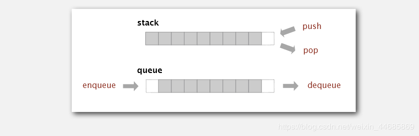
Stack, also known as stack, is a linear table with limited operation. A linear table that is restricted to insert and delete operations only at the end of the table. This end is called the top of the stack, and the other end is called the bottom of the stack. Inserting new elements into a stack is also called pushing, pushing or pressing. It is to put new elements on top of the stack to make it a new stack top element. Deleting elements from a stack is also called pushing out or pushing back. It is to delete the stack top elements and make the adjacent elements become new stack top elements.

As a data structure, stack is a special linear table which can only insert and delete at one end. It stores data according to the principle of first in and last out. The first in data is pressed into the bottom of the stack, and the last data is on the top of the stack. When it needs to read data, data will pop up from the top of the stack (the last data is read out by the first). The stack has a memory function. In the insertion and deletion of the stack, the pointer at the bottom of the stack does not need to be changed.
A stack is a special linear table that allows insertion and deletion at the same end. One end of the stack that allows insertion and deletion is called top, and the other end is bottom; the bottom of the stack is fixed, while the top of the stack is floating; when the number of elements in the stack is zero, it is called empty stack. Insertion is generally called PUSH, and deletion is called POP. The stack is also known as the first in first out table.

Stack can be used to store breakpoints in function calls, and stack is used in recursion!

Stack features:

Last in, first out, the last inserted element comes out first.

Python implementation

# The implementation of sequence table of stack

class Stack(object):
def __init__(self):
self.items = []

def isEmpty(self):
return self.items == []

def push(self, item):
return self.items.append(item)

def pop(self):
return self.items.pop()

def top(self):
return self.items[len(self.items)-1]

def size(self):
return len(self.items)

if __name__ == '__main__':
stack = Stack()
stack.push("Hello")
stack.push("World")
stack.push("!")
print(stack.size())
print(stack.top())
print(stack.pop())
print(stack.pop())
print(stack.pop())

# Result
3
!
!
World
Hello

# Implementation of link table of stack

class SingleNode(object):
def __init__(self, item):
self.item = item
self.next = None

class Stack(object):
def __init__(self):
self._head = None

def isEmpty(self):
return self._head == None

def push(self, item):
node = SingleNode(item)
node.next = self._head
self._head = node

def pop(self):
cur = self._head
self._head = cur.next
return cur.item

def top(self):
return self._head.item

def size(self):
cur = self._head
count = 0
while cur != None:
count += 1
cur = cur.next
return count

if __name__ == '__main__':
stack = Stack()
stack.push("Hello")
stack.push("World")
stack.push("!")
print(stack.size())
print(stack.top())
print(stack.pop())
print(stack.pop())
print(stack.pop())

# Result
3
!
!
World
Hello

queue
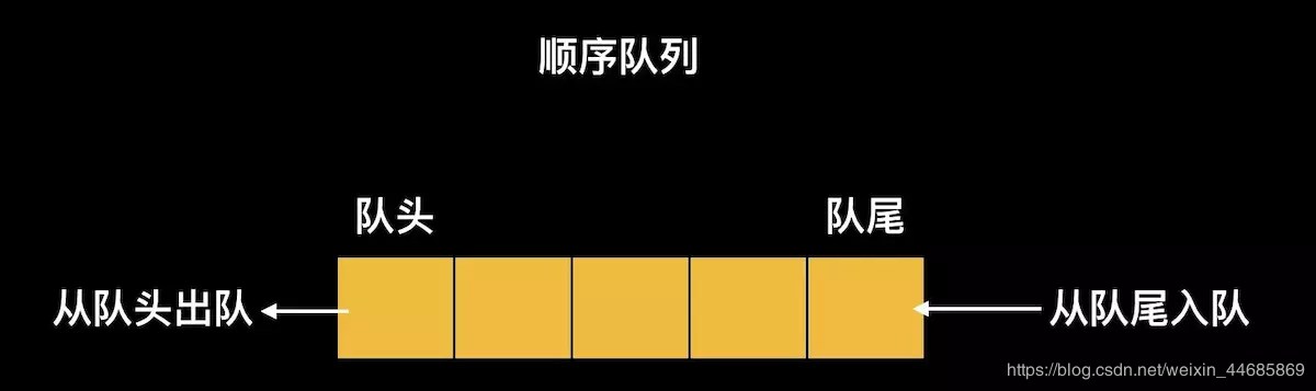
Queue is a kind of special linear table. The special thing is that it only allows deletion at the front end of the table and insertion at the rear end of the table. Like stack, queue is a kind of linear table with limited operation. The end of the insertion operation is called the end of the queue, and the end of the deletion operation is called the head of the queue. When there are no elements in the queue, it is called an empty queue.

The data elements of a queue are also called queue elements. Inserting a queue element into a queue is called queuing, and deleting a queue element from a queue is called queuing. Because queues can only be inserted at one end and deleted at the other end, only the elements that enter the queue first can be deleted from the queue first. Therefore, queues are also called FIFO first in first out linear tables

Characteristics of the queue:

First in, first out. The first element to insert comes first.
We can imagine that the first to buy tickets in line, the first to buy tickets, the last can only be at the end, not allowed to jump in line.

There are two basic operations of queue: to enter the queue and put a data at the end of the queue; to leave the queue and take an element from the head of the queue. Queue is also a kind of linear table data structure with limited operation. It has the characteristics of first in first out. It supports inserting elements at the end of the queue and deleting elements at the head of the queue.

The concept of queue is well understood, and the application of queue is also very extensive, such as loop queue, blocking queue, concurrent queue, priority queue, etc. It will be introduced below.

Sequence queue:
Sequence queue is what we often say FIFO (first in, first out) queue, which mainly includes: take the first element (first method), enter the queue (enqueue method), exit the queue (dequeue method), clear the queue (clear method), judge whether the queue is empty (empty method), get the queue length (length method). See the following source code for specific implementation. Similarly, when fetching the first element of the queue and getting out of the queue, you need to determine whether the next queue is empty.

class Queue:
"""
Sequential queue implementation
"""

def __init__(self):
"""
Initialize an empty queue because the queue is private
"""
self.__queue = []

def first(self):
"""
Get the first element of the queue
 : return: returns None if the queue is empty, otherwise returns the first element
"""
return None if self.isEmpty() else self.__queue[0]

def enqueue(self, obj):
"""
Queue elements
 : param obj: object to be queued
"""
self.__queue.append(obj)

def dequeue(self):
"""
Remove the first element from the queue
 : return: returns None if the queue is empty, or dequeued element
"""
return None if self.isEmpty() else self.__queue.pop(0)

def clear(self):
"""
Clear entire queue
"""
self.__queue.clear()

def isEmpty(self):
"""
Judge whether the queue is empty
 Return: bool value
"""
return self.length() == 0

def length(self):
"""
Get queue length
 And return
"""
return len(self.__queue)

Priority queue:
Priority queue is simply an ordered queue, and the sorting rule is the customized priority size. In the following code implementation, we mainly use the numerical value size to compare and sort. The smaller the numerical value is, the higher the priority will be. In theory, we should put the high priority first in the queue. It is worth noting that when I use list to implement, the order is reversed, i.e. the elements in list are from large to small. The advantage of this is that the time complexity of the first element of the queue and the two operations of outgoing queue is O(1), and the time complexity of only incoming queue operation is O(n). If we follow the order from small to large, we will have two time complexity O(n) and one time complexity O(1).

class PriorQueue:
"""
Priority queue implementation
"""

def __init__(self, objs=[]):
"""
Initialize priority queue, default queue is empty
 : parameter objs: object list initialization
"""
self.__prior_queue = list(objs)
#Sort from maximum to minimum with the minimum having the highest priority
 #Make the efficiency of "dequeue" O(1)
self.__prior_queue.sort(reverse=True)

def first(self):
"""
Get the highest priority element o of the priority queue (1)
: return: if the priority queue is empty, then None is returned; otherwise, the element with the highest priority is returned
"""
return None if self.isEmpty() else self.__prior_queue[-1]

def enqueue(self, obj):
"""
Add an element to the priority queue, O(n)
: param obj: object to be queued
"""
index = self.length()
while index > 0:
if self.__prior_queue[index - 1] < obj:
index -= 1
else:
break
self.__prior_queue.insert(index, obj)

def dequeue(self):
"""
Get the highest priority element from the priority queue, O(1)
: return: if the priority queue is empty, then None will be returned; otherwise, dequeued element will be returned
"""
return None if self.isEmpty() else self.__prior_queue.pop()

def clear(self):
"""
Clear entire priority queue
"""
self.__prior_queue.clear()

def isEmpty(self):
"""
Determine whether the priority queue is empty
 Return: bool value
"""
return self.length() == 0

def length(self):
"""
Get the length of the priority queue
 Return:
"""
return len(self.__prior_queue)

Loop queue:
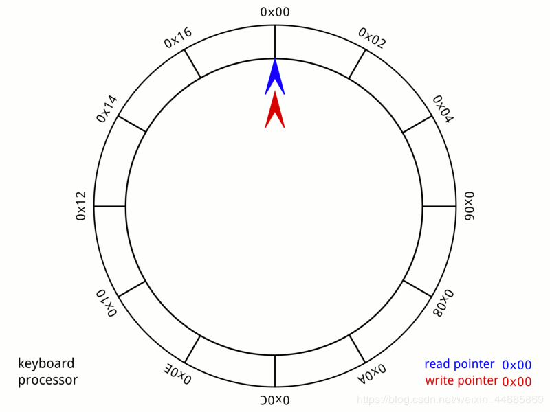
Circular queue is to connect the head and tail of ordinary queue to form a ring, and set the head and tail pointers respectively to indicate the head and tail of the queue. Every time we insert an element, the tail pointer moves backward one bit. Of course, the maximum length of our queue is defined in advance here. When we pop up an element, the head pointer moves backward one bit.

In this way, there is no delete operation in the list, only modify operation, so as to avoid the problem of high cost caused by deleting the previous nodes.

class Loopqueue:
'''
//Loop queue implementation
'''
def __init__(self, length):
self.head = 0
self.tail = 0
self.maxSize = length
self.cnt = 0
self.__list = [None]*length

def __len__(self):
'''
//Defining length
'''
return self.cnt

def __str__(self):
'''
//Define return value type
'''
s = ''
for i in range(self.cnt):
index = (i + self.head) % self.maxSize
s += str(self.__list[index])+' '
return s

def isEmpty(self):
'''
//Judge whether it is empty
'''
return self.cnt == 0

def isFull(self):
'''
//Judge whether it is full
'''
return self.cnt == self.maxSize

def push(self, data):
'''
//Additive elements
'''
if self.isFull():
return False
if self.isEmpty():
self.__list[0] = data
self.head = 0
self.tail = 0
self.cnt = 1
return True
self.tail = (self.tail+1)%self.maxSize
self.cnt += 1
self.__list[self.tail] = data
return True

def pop(self):
'''
//Pop-up elements
'''
if self.isEmpty():
return False
data = self.__list[self.head]
self.head = (self.head+1)%self.maxSize
self.cnt -= 1
return data

def clear(self):
'''
//Clear queue
'''
self.head = 0
self.tail = 0
self.cnt = 0
return True

Blocking queue
Blocking queue is a queue that supports two additional operations on the basis of queue.

The difference between a blocking (concurrent) queue and a normal queue is that when the queue is empty, the operation of getting elements from the queue will be blocked, or when the queue is full, the operation of adding elements to the queue will be blocked. Threads trying to get elements from an empty blocking queue will be blocked until other threads insert new elements into the empty queue. Similarly, threads trying to add new elements to a full blocking queue will also be blocked until other threads make the queue idle again, such as removing one or more elements from the queue, or completely emptying the queue

2 additional operations:
Support blocking insertion method: when the queue is full, the queue will block the thread of the inserted element until the queue is not satisfied.
The removal method that supports blocking: when the queue is empty, the thread that gets the element will wait for the queue to become non empty.

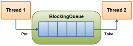
How to implement blocking queue? Of course, it depends on the lock, but how to lock it? A lock can be shared among three conditions: not empty, not full, all tasks done. For example, thread a, thread B, is now ready to put tasks to the queue. The maximum length of the queue is 5. When thread a is put, it is not finished. Thread B will start putting, and the queue will not be filled. Therefore, when thread a seizes the put right, it should add a lock to prevent thread B from operating on the queue. It is also important in the thread that the counting Jun often seen in ghost livestock area is increased by one after putting and decreased by one after get ting.

import threading #Introduce thread lock
import time
from collections import deque # Import queue


class BlockQueue:
def __init__(self, maxsize=0):
'''
//Three conditions of a lock (self.mutex, (self.not fu ll, self.not empty, self.all \,
//Max size (self.maxsize,self.unfinished)
'''
self.mutex = threading.Lock() # Thread locking
self.maxsize = maxsize 
self.not_full = threading.Condition(self.mutex)
self.not_empty = threading.Condition(self.mutex)
self.all_task_done = threading.Condition(self.mutex)
self.unfinished = 0

def task_done(self):
'''
//Task ﹣ done is called once after each put, and the number of calls cannot be more than the elements of the queue. Count the corresponding method,
unfinished<0 Time means call task_done There are more times than the elements of the list, and an exception is thrown.
'''
with self.all_task_done:
unfinish = self.unfinished - 1
if unfinish <= 0:
if unfinish < 0:
raise ValueError("The number of calls to task_done() is greater than the number of queue elements")
self.all_task_done.notify_all()
self.unfinished = unfinish

def join(self):
'''
//Blocking method is a very important method, but its implementation is not difficult. As long as the task is not completed, it always wait s (),
//When the count is unfinished > 0, wait () until unfinished=0 jumps out of the loop.
'''
with self.all_task_done:
while self.unfinished:
self.all_task_done.wait()

def put(self, item, block=True, timeout=None):
'''
block=True Block until a free slot is available, n If there is no free slot at that time, a complete exception will be thrown.
Block=False If an empty slot is immediately available, an entry is placed on the queue, otherwise a full exception is thrown (in this case, "timeout" is ignored).
//There is a vacancy, which is added to the unfinished task + 1 of the queue. At last, he needs to wake up not Fu empty. Notify(), because at first, he needs to lock when it is not full, and when it is full, he waits for not Fu full. Wait,
//There is something after put ting. Whenever an item is added to the queue, the thread notifying not empty of waiting for getting will be notified.
'''
with self.not_full:
if self.maxsize > 0:
if not block:
if self._size() >= self.maxsize:
raise Exception("The BlockQueue is full")
elif timeout is not None:
self.not_full.wait()
elif timeout < 0:
raise Exception("The timeout period cannot be negative")
else:
endtime = time.time() + timeout
while self._size() >= self.maxsize:
remaining = endtime - time.time()
if remaining <= 0.0:
raise Exception("The BlockQueue is full")
self.not_full.wait(remaining)
self.queue.append(item)
self.unfinished += 1
self.not_empty.notify()

def get(self, block=True, timeout=None):
'''
//If the optional args "block" is True and timeout is None, block if necessary until a project is available.
//If the timeout is a non negative number, it blocks n seconds, and if there are no items to get () within that time, a null exception is thrown.
//Otherwise, 'block' is False. If it is available immediately, an empty exception will be thrown, in which case the timeout will be ignored.
//In the same way, wake up not full.notify
'''
with self.not_empty:
if not block:
if self._size() <= 0:
raise Exception("The queue is empty and you can't call get ()")
elif timeout is None:
while not self._size():
self.not_empty.wait()
elif timeout < 0:
raise ValueError("The timeout cannot be an integer")
else:
endtime = time.time() + timeout
remaining = endtime - time.time()
if remaining <= 0.0:
raise Exception("The BlockQueue is empty")
self.not_empty.wait(remaining)
item = self._get()
self.not_full.notify()
return item

Block queue extract address

Concurrent queues:
JDK provides two sets of implementations on concurrent queues,

One is that the high-performance queue represented by ConcurrentLinkedQueue is non blocking,

One is the blocking Queue represented by the BlockingQueue interface, which inherits from the Queue.

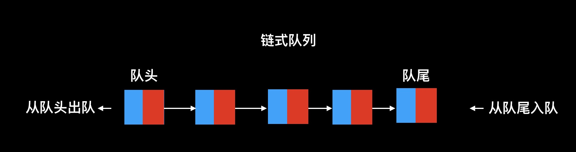
Chain queue:
When a chain queue is created, the data field and next field of the node pointed to by the front and rear pointer of the queue are empty.

class QueueNode():
def __init__(self):
self.data = None
self.next = None
class LinkQueue():
def __init__(self):
tQueueNode = QueueNode()
self.front = tQueueNode
self.rear = tQueueNode
'''Judge whether it is empty'''
def IsEmptyQueue(self):
if self.front == self.rear:
iQueue = True
else:
iQueue = False
return iQueue
'''Incoming queue'''
def EnQueue(self,da):
tQueueNode = QueueNode()
tQueueNode.data = da
self.rear.next = tQueueNode
self.rear = tQueueNode
print("The current entry elements are:",da)
'''Outgoing queue'''
def DeQueue(self):
if self.IsEmptyQueue():
print("Queue is empty")
return
else:
tQueueNode = self.front.next
self.front.next = tQueueNode.next
if self.rear == tQueueNode:
self.rear = self.front
return tQueueNode.data
def GetHead(self):
if self.IsEmptyQueue():
print("Queue is empty")
return
else:
return self.front.next.data
def CreateQueueByInput(self):
data = input("Please enter the element (enter OK,#End)")
while data != "#":
self.EnQueue(data)
data = input("Please enter the element (enter OK,#End)")
'''Traversal of all elements in the sequence queue'''
def QueueTraverse(self):
if self.IsEmptyQueue():
print("Queue is empty")
return
else:
while self.front != self.rear:
result = self.DeQueue()
print(result,end = ' ')
lq = LinkQueue()
lq.CreateQueueByInput()
print("The elements in the queue are:")
lq.QueueTraverse()

# Result

//Please enter the element (enter OK,#End) 5
//The current entry element is: 5
//Please enter the element (enter OK,#End) 8
//The current entry element is: 8
//Please enter the element (enter OK,#End) 9
//The current entry element is: 9
//Please enter the element (enter OK,#End)#
The elements of the queue are:
5 8 9

Linked list
Linked list is a kind of non continuous and non sequential storage structure on physical storage unit. The logical order of data elements is realized by the pointer link order in linked list. The list consists of a series of nodes (each element in the list is called a node), which can be generated dynamically at runtime. Each node consists of two parts: one is the data field for storing data elements, the other is the pointer field for storing the address of the next node. Compared with the linear table sequential structure, the operation is complex. Because it does not have to be stored in order, the chain table can achieve O(1) complexity when inserting, which is much faster than the other linear table sequence table. However, it takes O(n) time to find a node or access a specific number of nodes, while the corresponding time complexity of linear table and sequence table are O(logn) and O(1), respectively.

Linked list is a kind of storage structure which is not continuous and sequential in physical storage structure. The logical order of data elements is realized by the order of pointer link in linked list.

The structure of the chain list is various. At that time, there were usually two types:

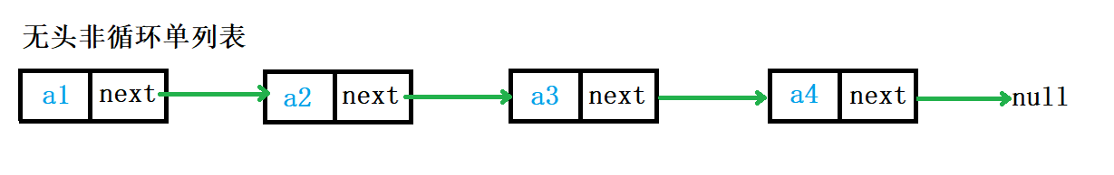
Headless one-way acyclic list: it is simple in structure and will not be used to store data alone. In fact, it is more a substructure of other data structures, such as hash bucket and so on.
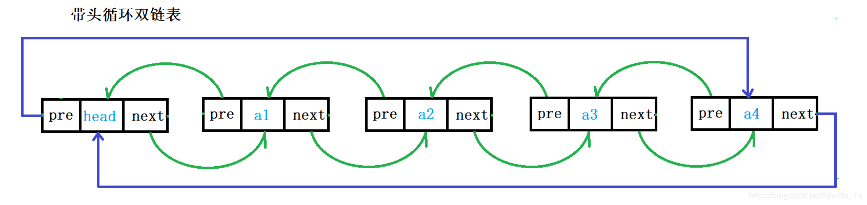
                   . In fact, most of the data structures of linked list are two-way circular linked list. Although the structure is complex, it will bring many advantages after using the code implementation, but the implementation is simple.

Advantages of linked list
The efficiency of insertion and deletion is high. Only changing the pointer can insert and delete.
The memory utilization is high, and the memory will not be wasted. The small discontinuous space in the memory can be used, and the space can be created only when it is needed. The size is not fixed and the expansion is flexible.

Disadvantages of linked list
The efficiency of lookup is low, because the linked list traverses the lookup backward from the first node.

AAA original link

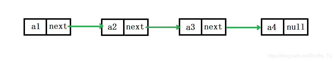
One-way linked list
One way linked list (single linked list) is a kind of linked list, which is characterized by that the link direction of the linked list is one-way, and the access to the linked list starts from the head through sequential reading; the linked list is a list constructed by using pointers; also known as node list, because the linked list is assembled by nodes; each node has a pointer member variable to the next node in the list ; list is composed of nodes. The head pointer points to the first node that becomes the header node, and terminates at the last pointer that points to NULL.

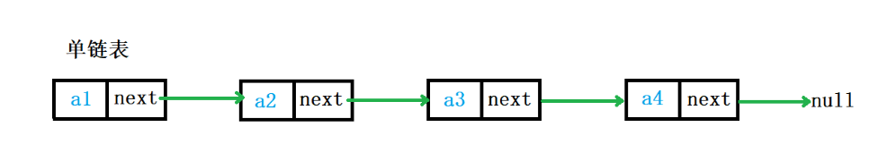
In a single chain table, each node has only a pointer to the next node, so it can't be traced back. It is suitable for adding and deleting nodes.

class Node(object):
"""node"""

def __init__(self, elem):
self.elem = elem
self.next = None # Initial setting next node is empty

'''
//The above defines a node class. Of course, you can also directly use some of python's structures. For example, through the tuple (elem, None)
'''


# Next, create a single chain table and implement its functions


class SingleLinkList(object):
"""Single linked list"""

def __init__(self, node=None): # Use a default parameter to receive when the header node is passed in. If there is no incoming, the header node is empty by default
self.__head = node

def is_empty(self):
'''Whether the list is empty'''
return self.__head == None

def length(self):
'''Length of linked list'''
# cur Cursor, used to move traversal node
cur = self.__head
# count Number of records
count = 0
while cur != None:
count += 1
cur = cur.next
return count

def travel(self):
'''Traverse the entire list'''
cur = self.__head
while cur != None:
print(cur.elem, end=' ')
cur = cur.next
print("\n")

def add(self, item):
'''Add elements to the head of the list'''
node = Node(item)
node.next = self.__head
self.__head = node

def append(self, item):
'''Add elements at the end of the list'''
node = Node(item)
# Due to special circumstances, when the list is empty, there is no next，So we need to make a judgment
if self.is_empty():
self.__head = node
else:
cur = self.__head
while cur.next != None:
cur = cur.next
cur.next = node

def insert(self, pos, item):
'''Add element at specified location'''
if pos <= 0:
# If pos If the position is 0 or before, it should be done by head insertion
self.add(item)
elif pos > self.length() - 1:
# If pos If the location is longer than the original list, it should be done as tail insertion
self.append(item)
else:
per = self.__head
count = 0
while count < pos - 1:
count += 1
per = per.next
# When the loop exits, pre point pos-1 position
node = Node(item)
node.next = per.next
per.next = node

def remove(self, item):
'''Delete node'''
cur = self.__head
pre = None
while cur != None:
if cur.elem == item:
# First, judge whether the node is the head node
if cur == self.__head:
self.__head = cur.next
else:
pre.next = cur.next
break
else:
pre = cur
cur = cur.next

def search(self, item):
'''Find whether the node exists'''
cur = self.__head
while not cur:
if cur.elem == item:
return True
else:
cur = cur.next
return False


if __name__ == "__main__":

# node = Node(100) # First create a node and pass it in

ll = SingleLinkList()
print(ll.is_empty())
print(ll.length())

ll.append(3)
ll.add(999)
ll.insert(-3, 110)
ll.insert(99, 111)
print(ll.is_empty())
print(ll.length())
ll.travel()
ll.remove(111)
ll.travel()

Two way linked list
Double linked list is also called double linked list. It is a kind of linked list. There are two pointers in each data node, pointing to direct successor and direct precursor respectively. Therefore, starting from any node in the two-way linked list, you can easily access its predecessor and successor nodes. Generally, we construct a bidirectional circular list.

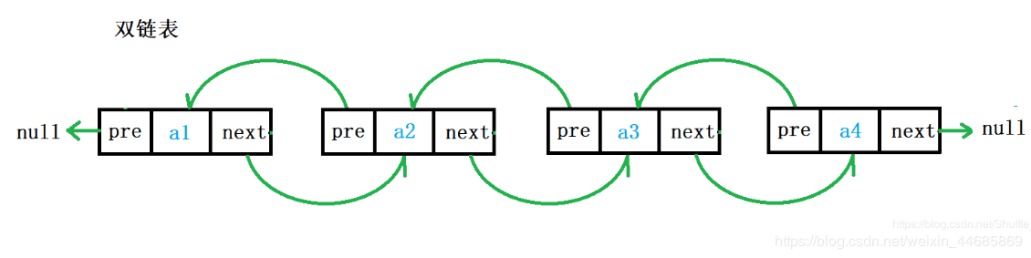
Each node in the double linked list has both a pointer to the next node and a pointer to the previous node. It can quickly find the previous node of the current node, which is suitable for the situation where the node value needs to be searched in two directions.

Similar to a single chain table, it just adds a pointer to the previous element.

class Node(object):
def __init__(self,val,p=0):
self.data = val
self.next = p
self.prev = p

class LinkList(object):
def __init__(self):
self.head = 0

def __getitem__(self, key):

if self.is_empty():
print 'linklist is empty.'
return

elif key <0 or key > self.getlength():
print 'the given key is error'
return

else:
return self.getitem(key)

 

def __setitem__(self, key, value):

if self.is_empty():
print 'linklist is empty.'
return

elif key <0 or key > self.getlength():
print 'the given key is error'
return

else:
self.delete(key)
return self.insert(key)

def initlist(self,data):

self.head = Node(data[0])

p = self.head

for i in data[1:]:
node = Node(i)
p.next = node
node.prev = p
p = p.next

def getlength(self):

p = self.head
length = 0
while p!=0:
length+=1
p = p.next

return length

def is_empty(self):

if self.getlength() ==0:
return True
else:
return False

def clear(self):

self.head = 0


def append(self,item):

q = Node(item)
if self.head ==0:
self.head = q
else:
p = self.head
while p.next!=0:
p = p.next
p.next = q
q.prev = p


def getitem(self,index):

if self.is_empty():
print 'Linklist is empty.'
return
j = 0
p = self.head

while p.next!=0 and j <index:
p = p.next
j+=1

if j ==index:
return p.data

else:

print 'target is not exist!'

def insert(self,index,item):

if self.is_empty() or index<0 or index >self.getlength():
print 'Linklist is empty.'
return

if index ==0:
q = Node(item,self.head)

self.head = q

p = self.head
post = self.head
j = 0
while p.next!=0 and j<index:
post = p
p = p.next
j+=1

if index ==j:
q = Node(item,p)
post.next = q
q.prev = post
q.next = p
p.prev = q


def delete(self,index):

if self.is_empty() or index<0 or index >self.getlength():
print 'Linklist is empty.'
return

if index ==0:
q = Node(item,self.head)

self.head = q

p = self.head
post = self.head
j = 0
while p.next!=0 and j<index:
post = p
p = p.next
j+=1

if index ==j:
post.next = p.next
p.next.prev = post

def index(self,value):

if self.is_empty():
print 'Linklist is empty.'
return

p = self.head
i = 0
while p.next!=0 and not p.data ==value:
p = p.next
i+=1

if p.data == value:
return i
else:
return -1


l = LinkList()
l.initlist([1,2,3,4,5])
print l.getitem(4)
l.append(6)
print l.getitem(5)

l.insert(4,40)
print l.getitem(3)
print l.getitem(4)
print l.getitem(5)

l.delete(5)
print l.getitem(5)

l.index(5)

# Result
5
6
4
40
5
6

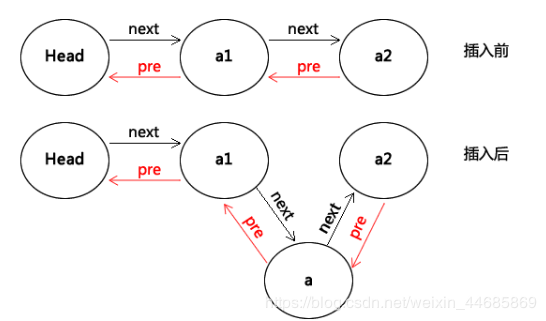
Advantages of double linked list over single linked list:

When deleting a node in a single chain table, you must get the precursor of the node to be deleted. The method to get the precursor is to save the precursor of the current node all the way when locating the node to be deleted. In this way, the total movement of the pointer is 2n times. If you use a double chain table, you do not need to locate the precursor, so the total movement of the pointer is n times.
The same is true for    searching. We can use the dichotomy idea to do the search from the beginning to the back and from the end to the front at the same time, so the efficiency can also be doubled. But why is the use of single linked list more than that of double linked list in the market? From the perspective of storage structure, each node of double linked list has one more pointer than that of single linked list. If the length is n, it needs space of n * light (32 bits are 4 bytes, 64 bits are 8 bytes). This is not applicable in some applications with low time efficiency. Because it takes up more than 1 / 3 of the space of single linked list, designers will change space in one time.

Reversal of one way linked list
Name as it means: reverse the single chain table.
Example: how to reverse 1234 to 4321
1234 - > 2134 - > 2314 - > 2341 - > 3241 - > 3421 - > 4321. It's too hard. It's like bubble sorting
It should be to put the number after N in front every time, 1234n - > 1n234 - > 21n34 - > 321n4 - > 4321n

Then we'll implement it in Python

The first method is cyclic method
The idea of the loop method is to establish three variables, pointing to the current node, the previous node of the current node, and the new head node. Starting from the head, each loop reverses the direction of the two adjacent nodes. After the whole chain list is traversed, the direction of the chain list is reversed.

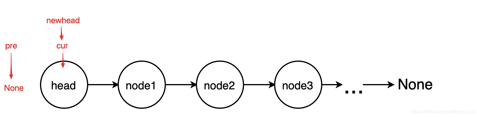
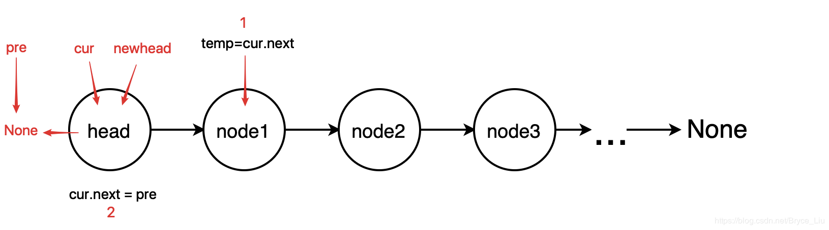
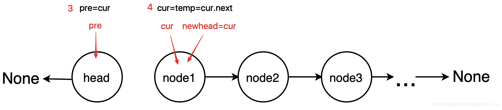
class ListNode:
def __init__(self, x):
self.val = x
self.next = None


def reverse(head): # The method of loop reverses the linked list
if head is None or head.next is None:
return head
# Define the initial state of the reversal
pre = None
cur = head
newhead = head
while cur:
newhead = cur
tmp = cur.next
cur.next = pre
pre = cur
cur = tmp
return newhead

if __name__ == '__main__':
head = ListNode(1) # Test code
p1 = ListNode(2) # Create linked list 1->2->3->4->None;
p2 = ListNode(3)
p3 = ListNode(4)
head.next = p1
p1.next = p2
p2.next = p3
p = reverse(head) # Output list 4->3->2->1->None
while p:
print(p.val)
p = p.next

The second is recursive method

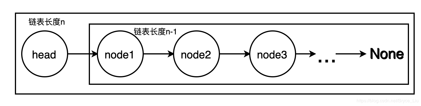
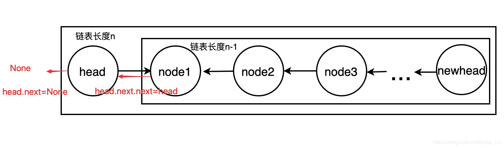
According to the concept of recursion, we only need to pay attention to the base case condition of recursion, that is, the exit of recursion or the termination condition of recursion, as well as the relationship between the linked list with length N and the linked list with length n-1
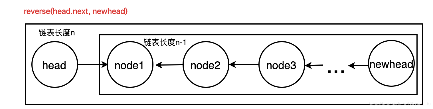
The reverse result of the n-1 chain list only needs to reverse the n-1 chain list, change the last point of the chain list to the head of the n chain list, and make the head point to None (or add the head node of the n chain list between the chain list and None)
That is, to reverse the n-1 list, first reverse the n-1 list, and then operate to reverse the relationship between the good list and the head node. As for how to reverse the n-1 length list, just split it into the node1 and n-2 list

class ListNode:
def __init__(self, x):
self.val = x
self.next = None


def reverse(head, newhead): # Recursion head Is the head node of the original list, newhead Is the head node of the reverse linked list
if head is None:
return
if head.next is None:
newhead = head
else:
newhead = reverse(head.next, newhead)
head.next.next = head
head.next = None
return newhead

if __name__ == '__main__':
head = ListNode(1) # Test code
p1 = ListNode(2) # Create linked list 1->2->3->4->None
p2 = ListNode(3)
p3 = ListNode(4)
head.next = p1
p1.next = p2
p2.next = p3
newhead = None
p = reverse(head, newhead) # Output list 4->3->2->1->None
while p:
print(p.val)
p = p.next

array
An array is an ordered sequence of elements. If you name a collection of a limited number of variables of the same type, the name is an array name. The variables that make up an array are called the components of the array, also called the elements of the array, and sometimes called subscript variables. The number used to distinguish the elements of an array is called a subscript. Array is a kind of form in which several elements of the same type are organized in an unordered form for the convenience of processing. These unordered collections of like data elements are called arrays.
An array is a collection used to store data of the same type.

Python has no built-in support for arrays, but you can use Python lists instead.

One-dimensional array
One dimensional array is the simplest array, whose logical structure is linear table. To use a one-dimensional array, it needs to go through the process of definition, initialization and application.

In the declaration format of array, "data type" is the data type of declaration array element, which can be any data type in java language, including simple type and structure type. Array name is used to unify the names of these same data types. Its naming rules are the same as those of variables.
After an array is declared, the next step is to allocate the memory required by the array. At this time, the operator new must be used, where "number" is to tell the compiler how many elements the declared array should hold, so the new operator is to inform the compiler to allocate a space for the array in internal storage according to the number in brackets. Using the new operator to allocate memory space for array elements is called dynamic allocation.

Two-dimensional array
The array described above has only one subscript, which is called one-dimensional array, and its array elements are also called single subscript variables. In practical problems, many quantities are two-dimensional or multi-dimensional, so multi-dimensional array elements have multiple subscripts to identify its position in the array, so they are also called multi subscript variables.

The concept of two-dimensional array is two-dimensional, that is to say, its subscript changes in two directions, and the position of subscript variable in the array is also in a plane, rather than just a vector like one-dimensional array. However, the actual hardware memory is continuously addressed, that is to say, the memory cells are arranged in linear one dimension. There are two ways to store two-dimensional arrays in one-dimensional memory: one is to arrange them in rows, that is, to put one row in sequence and then put the second row. The other is to arrange by column, that is, put one column in sequence and then put the second column. In C, two-dimensional arrays are arranged in rows. In the above section, you can store lines a[0], a[1] and a[2] in sequence. There are four elements in each row in turn. Because array A is described as
int type, which takes up two bytes of memory space, so each element takes up two bytes (each cell in the figure is a byte).

Three dimensional array
Three dimensional array refers to the array structure with three dimensions. 3D array is the most common multidimensional array, which is widely used because it can be used to describe the position or state in 3D space.
A three-dimensional array is an array with three dimensions. It can be considered that three independent parameters are used to describe the contents stored in the array, but more importantly, the subscript of the array is composed of three different parameters.
The concept of array is mainly used in programming, which is different from the concepts of vector and matrix in mathematics. It mainly shows that the elements in array can be any same data type, including vector and matrix.
The access to arrays is usually through subscripts. In a three-dimensional array, the subscript of the array is composed of three numbers, through which the contents of the array are accessed.

Character array
The array used to store the amount of characters is called a character array.
The character array type description takes the same form as the numerical array described earlier. For example: char c[10]; because of the common character type and integer type, it can also be defined as int c[10], but at this time, each array element occupies 2 bytes of memory.
The character array can also be a two-dimensional or multi-dimensional array, for example: char c[5][10]; that is, a two-dimensional character array

Dictionary implementation principle NSDictionary
The dict object in Python indicates that it is a primitive Python data type, stored in the way of key value pairs. Its Chinese name is translated into a dictionary. As the name implies, it will have a high efficiency to find the corresponding value through the key name. The time complexity is at constant level O(1)

Low level implementation of dict
In Python, dictionaries are implemented through hash tables. In other words, the dictionary is an array, and the index of the array is obtained after the key is hashed.

Hashtable
It is a data structure accessed directly according to key value. It accesses records by mapping key values to a location in the table to speed up the search.
This mapping function is called hash function, and the array of records is called hash table.
Given table M, there is function f(key). For any given key value key, if the address of the record containing the key in the table can be obtained after the function is substituted, then table M is called Hash table
Function f(key) is a hash function.

>>> map(hash, (0, 1, 2, 3)) 

[0, 1, 2, 3] 

>>> map(hash, ("namea", "nameb", "namec", "named")) 

[-1658398457, -1658398460, -1658398459, -1658398462] 

Hash concept: the essence of hash table is an array. Each element in the array is called a bin, in which key value pairs are stored.

hash function
Hash function is a mapping, so the setting of hash function is very flexible, as long as the hash function value obtained by any keyword falls within the range allowed by the table length;
Not all inputs correspond to only one output, that is to say, hash function can not be made into a one-to-one mapping relationship, and its essence is a many to one mapping, which leads to the following concept conflict.

conflict

As long as it's not a one-to-one mapping relationship, the conflict will inevitably occur, or the extreme example above. At this time, a new employee with employee number 2 is added, regardless of the size of our array. According to the previous hash function, the hash value of employee with job number 2 is also 2, which is the same as that of employee with 10000000000001. This is a conflict, aiming at different solutions Three different solutions are proposed.

Conflict resolution

Open address
Open address means that in addition to the address obtained by hash function, other addresses are also available when there is a conflict. Common methods of open address thinking include linear detection and re hashing, and secondary detection and re hashing. These methods are all solutions in the case that the first choice is occupied.

double hashing
This method specifies multiple hash functions in order. Each time a query is made, the hash function is called in order. When the first call is empty, the return function does not exist. When the key is called, the value is returned.

Chain address method
All records with the same key hash value exist in the same linear linked list, so that no other hash address is occupied. The same hash value can be found by traversing in order on a linked list.

Public overflow area
The basic idea is: no matter what the hash address they get from the hash function is, once there is a conflict, they will fill in the overflow table.

Loading factor α
In general, the average lookup length of a hash table with the same conflict handling method depends on the load factor of the hash table. The load factor of hash table is defined as the number of records filled in the table and the wallpaper of hash table length, which indicates the full degree of hash table. Intuitively, the smaller α is, the less likely conflict will occur, and vice versa. Generally, 0.75 is suitable, involving mathematical derivation.

Hash stored procedure

1. Calculate its hash value h according to the key.

2. If the number of boxes is n, the key value pair should be placed in the (H% n) box.

3. If there are already key value pairs in the box, open addressing method or zipper method will be used to solve the conflict.

When using zipper method to solve hash conflict, each box is actually a linked list, and all key value pairs belonging to the same box will be arranged in the linked list. The hash table also has an important attribute: load factor, which is used to measure the empty / full degree of the hash table. To some extent, it can also reflect the efficiency of the query. The formula is: load factor = total key value logarithm / number of boxes the larger the load factor is, which means that the fuller the hash table is, the more likely it is to cause conflicts and the lower the performance. Therefore, generally speaking, when the load factor is greater than a certain constant (maybe 1, or 0.75, etc.), the hash table will be automatically expanded. When the hash table is automatically expanded, it will generally create boxes with twice the original number. Therefore, even if the hash value of the key is unchanged, the result of retrieving the number of boxes will change. Therefore, the storage location of all key value pairs may change. This process is also called rehash. The capacity expansion of hash table is not always able to effectively solve the problem of too large load factor. Assuming that the hash values of all keys are the same, their positions will not change even after the expansion. Although the load factor will be reduced, the length of the linked list actually stored in each bin does not change, so the query performance of the hash table cannot be improved. Based on the above summary, careful friends may find two problems with hash tables:

1. If there are many boxes in the hash table, it is necessary to re hash and move the data when expanding the capacity, which has a great impact on the performance.

2. If the hash function design is unreasonable, the hash table will become a linear table in extreme cases, with extremely low performance.

All immutable built-in types in Python are hashable.
Variable types (such as lists, dictionaries, and collections) are not hashable and therefore cannot be used as keys to dictionaries.

tree
Tree is a kind of data structure, which consists of n (n > = 1) finite nodes to form a set with hierarchical relationship. It's called "tree" because it looks like an upside down tree, that is, it's root up and leaf down. It has the following characteristics:
Each node has zero or more child nodes. A node without a parent node is called a root node. Each non root node has only one parent node. In addition to the root node, each child node can be divided into multiple disjoint subtrees;

Tree is an important non-linear data structure. Intuitively, it is a structure of data elements (called nodes in the tree) organized according to branch relations, much like the tree in nature.

Tree definition:
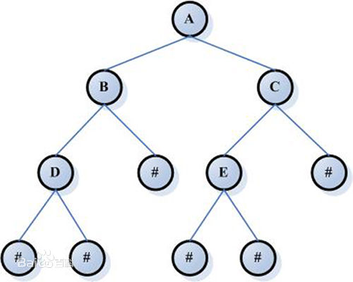
A tree is a hierarchical collection of nodes or vertices connected by edges. A tree cannot have loops, and only nodes and their descendent or child nodes have edges. Two child nodes of the same parent cannot have any edge between them. Each node can have a parent unless it is the top node, also known as the root node. Each tree can only have one root node. Each node can have zero or more children. In the following figure, a is the root node, and B, C, and D are the children of A. We can also say that a is the parent node of B, C and D. B. C and D are called siblings because they are from the same parent node a.

Tree species:

Unordered tree: there is no order relationship between any node's children in the tree. This tree is called unordered tree, also called free tree;
Ordered tree: any node in the tree has an order relationship between its children, which is called an ordered tree;
Binary tree: a tree with at most two subtrees per node is called a binary tree;
Complete binary tree
Full two fork tree
Huffman tree: the shortest binary tree with weight path is called Huffman tree or optimal binary tree;

Depth of tree:

The root node level of a tree is defined as 1, and the level of other nodes is the parent node level plus 1. The maximum value of the hierarchy of all nodes in a tree is called the depth of the tree.

Binary tree, full binary tree, complete binary tree
Binary tree is a kind of special tree: it is either empty. In a binary tree, each node has at most two child nodes, which are generally called left child nodes and right child nodes (or left child and right child nodes). Moreover, the subtrees of a binary tree can be divided into left and right ones, and their order cannot be reversed arbitrarily.

Full binary tree: in a binary tree, if all branch nodes have left child and right child nodes, and the leaf nodes are concentrated at the lowest level of the binary tree, such a tree is called full binary tree

Complete binary tree: if the degree of nodes in the lowest two layers of a binary tree can be less than 2 at most, and the leaf nodes in the lowest layer are arranged on the leftmost position of the layer in turn, it is called a complete binary tree

Difference: a full binary tree is a special case of a complete binary tree, because a full binary tree is full, but it does not mean full at all. So you should also imagine the form. Fullness refers to that each node outside the leaf node has two children, and the full meaning is that the last layer is not full, not full.

Two fork tree

In computer science, a binary tree is a tree structure in which each node has at most two subtrees. Generally, subtrees are called left subtree s and right subtree s. Binary tree is often used to implement binary search tree and binary heap.

Binary tree is defined recursively. Its nodes are divided into left and right subtrees. Logically, binary tree has five basic forms:

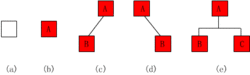
(1) Empty binary tree - as shown in figure (a);
(2) A two tree with only one root - as shown in Fig. (b);
(3) Only the left subtree - as shown in figure (1);
(4) Only the right subtree - as shown in figure (3);
(5) Complete binary tree - as shown in figure (3).

Note: Although there are many similarities between a binary tree and a tree, a binary tree is not a special case of a tree. [1]

hash tree
Hash tree (or hash tree) is a kind of persistent data structure, which can be used to implement collection and mapping, aiming to replace hash table in pure functional programming. In its basic form, the hash tree stores the hash value of its key (considered as a bit string) in the trie, where the actual key and (optionally) value are stored in the "final" node of the trie

What is prime: a number that can only be divided by 1 and itself.

Why prime numbers: because the number of consecutive integers that can be "distinguished" by N different prime numbers is the same as the product of these prime numbers.

That is to say, if there are 2.1 billion numbers, we can find the corresponding number even if we only need to calculate the bottom 10 times.
So hash tree is a tree for searching.

For example:
From two consecutive prime numbers, 10 consecutive prime numbers can distinguish about M(10) =23571113171923*29= 6464693230 numbers, which has exceeded the expression range of 32 bit integers commonly used in computers. One hundred prime numbers can distinguish about M(100) = 4.711930 times the 219 power of 10.
According to the current CPU level, 100 times of integer division operation is hardly difficult. In practical applications, the overall operation speed often depends on the number and time of key words loaded into memory by nodes. Generally speaking, the loading time is determined by the size of the key words and the hardware; under the same type of key words and the same hardware conditions, the actual overall operation time mainly depends on the loading times. There is a direct relationship between them.

AAA hash tree reference origin

B-tree/B+tree
Btree
Btree is a kind of multi-channel self balanced search tree, which is similar to the ordinary binary tree, but Btree allows each node to have more children. The schematic diagram of Btree is as follows:

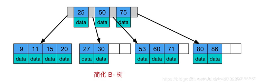
From the above figure, we can see some characteristics of Btree:

All key values are distributed throughout the tree
Any keyword appears and only appears in one node
Search may end at non leaf nodes
One search in the whole set of keywords, performance approaching binary search algorithm

B+tree

B + tree is a variant of B tree and a multi-channel balanced search tree. The schematic diagram of B + tree is as follows:

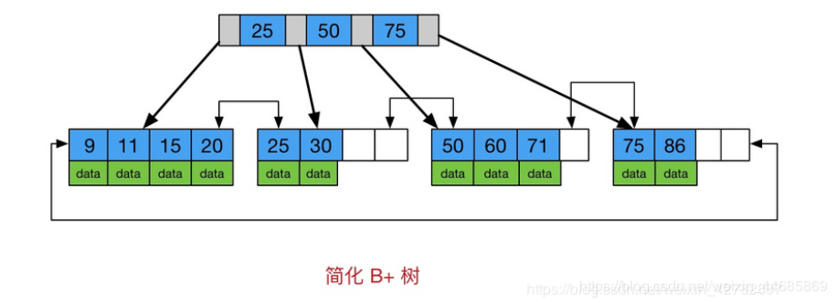
It can be seen from the figure that the characteristics of B+tree are also the differences between B+tree and B+tree

All keywords are stored in leaf nodes, while non leaf nodes do not store real data
Added a chain pointer for all leaf nodes, only one
Conclusion: in the index structure of data storage, Btree is more inclined to store data in vertical depth and B+tree is more inclined to store data in horizontal breadth.

Reference original address of AAAbtree