01 reading guidance

This course is Baidu's official zero basic in-depth learning course. It is mainly for students who have no in-depth learning technology foundation or weak foundation. It helps everyone realize the leap from 0 to 1 + in the field of in-depth learning. From this course, you will learn:

1. Deep learning of basic knowledge

2. Neural network construction and gradient descent algorithm implemented by numpy

3. Principle and practice of main directions in the field of computer vision

4. Principle and practice of main directions in natural language processing

5. Principle and practice of personalized recommendation algorithm

This week is the fourth week of the lecture. Sun Gaofeng, senior R & D Engineer of Baidu deep learning technology platform department, begins to explain the task of image classification in computer vision.

02 overview of image classification

Image classification is to distinguish different kinds of images according to the semantic information of images. It is an important basic problem in computer vision. It is also the basis of other high-level visual tasks such as object detection, image segmentation, object tracking, behavior analysis, face recognition and so on. Image classification has a wide range of applications in many fields, such as: face recognition and intelligent video analysis in the field of security, traffic scene recognition in the field of transportation, content-based image retrieval and album automatic classification in the field of Internet, image recognition in the field of medicine, etc.

The previous section mainly introduces some basic modules of convolutional neural network. In this section, based on ichallenge PM, the classic convolutional neural network in the field of image classification is analyzed, and how to use these basic modules to build convolutional neural network to solve the problem of image classification is introduced. The following convolutional neural networks are covered:

• LeNet: Yan LeCun and others first applied convolutional neural network to image classification task in 1998 [1], and achieved great success in handwritten digit recognition task.

• Alex net: Alex Krizhevsky and others put forward Alex net [2] in 2012 and applied it to the large-scale image data set ImageNet, winning the 2012 ImageNet Large Scale Visual Recognition Challenge (ILSVRC).

• VGG: Simonyan and Zisserman proposed the VGG network structure in 2014 [3], which is one of the most popular convolutional neural networks at present. Because of its simple structure and strong application, it is widely welcomed by researchers.

• GoogLeNet: Christian Szegedy and others put forward GoogLeNet[4] in 2014 and won the 2014 ImageNet championship.

• ResNet: Kaiming He et al. Proposed ResNet[5] in 2015. By introducing residual module to deepen the network layer, the recognition error rate on the Imagenet data set was reduced to 3.6%, which exceeded the level of human eye recognition. ResNet's design idea deeply influenced the later design of deep neural network.

03 LeNet

LeNet is one of the earliest convolutional neural networks [1]. In 1998, Yan LeCun first applied LeNet convolutional neural network to image classification, and achieved great success in handwritten digit recognition. LeNet extracts image features through continuous use of the combination of convolution and pooling layers. Its architecture is shown in Figure 1. Here is the LeNet-5 model in the author's paper:

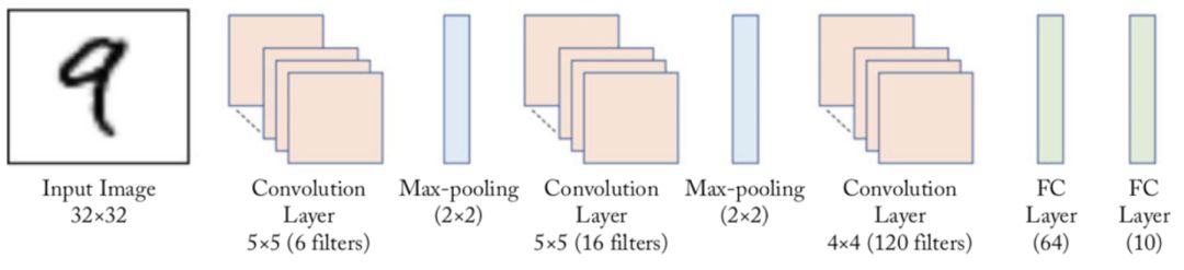
Figure 1: schematic diagram of LeNet model network structure

• The first round of convolution and pooling: convolution extracts the feature patterns contained in the image (activation function uses sigmoid), and the image size is reduced from 32 to 28. Through the pool layer, the sensitivity of the output feature map to the spatial position can be reduced, and the image size can be reduced to 14.

• The second round of convolution and pooling: the convolution operation reduces the image size to 10 and becomes 5 after pooling.

• The third round of convolution: input the feature image extracted by the third convolution into the full connection layer. The number of output neurons in the first full connection layer is 64, and the number of output neurons in the second full connection layer is the number of classification labels, and the size of handwritten digit recognition is 10. Then the prediction probability of each category can be calculated by using Softmax activation function.

[prompt]:

How to use the output characteristic graph of convolution layer as the input of full connection layer?

The output data format of the convolution layer is that when the full connection layer is input, the data will be flattened automatically,

That is, for each sample, it is automatically converted into a vector of length,

Among them, the data dimension of a mini batch becomes a two-dimensional vector.

03 application of lenet in handwritten digit recognition

The implementation code of LeNet network is as follows:

# Import required packages
import paddle
import paddle.fluid as fluid
import numpy as np
from paddle.fluid.dygraph.nn import Conv2D, Pool2D, FC

# Define the LeNet network structure
class LeNet(fluid.dygraph.Layer):
    def __init__(self, name_scope, num_classes=1):
        super(LeNet, self).__init__(name_scope)
        name_scope = self.full_name()
        # Create convolution and pooling layer blocks, each convolution layer uses the Sigmoid activation function, followed by a 2x2 pooling
        self.conv1 = Conv2D(name_scope, num_filters=6, filter_size=5, act='sigmoid')
        self.pool1 = Pool2D(name_scope, pool_size=2, pool_stride=2, pool_type='max')
        self.conv2 = Conv2D(name_scope, num_filters=16, filter_size=5, act='sigmoid')
        self.pool2 = Pool2D(name_scope, pool_size=2, pool_stride=2, pool_type='max')
        # Create the third volume layer
        self.conv3 = Conv2D(name_scope, num_filters=120, filter_size=4, act='sigmoid')
        # To create a full connection layer, the number of output neurons in the first full connection layer is 64, and the number of output neurons in the second full connection layer is the number of categories with split labels
        self.fc1 = FC(name_scope, size=64, act='sigmoid')
        self.fc2 = FC(name_scope, size=num_classes)
    # Forward computing process of network
    def forward(self, x):
        x = self.conv1(x)
        x = self.pool1(x)
        x = self.conv2(x)
        x = self.pool2(x)
        x = self.conv3(x)
        x = self.fc1(x)
        x = self.fc2(x)
        return x

The result shows that the accuracy of LeNet in MNIST verification data set is over 92%. So what about other data sets? Let's verify it with the eye disease recognition data set ichallenge PM.

Application of 04LeNet in ichallenge PM

iChallenge PM is a medical data set about pathological myopia (PM) jointly held by Baidu brain and Zhongshan eye center of Sun Yat sen University. It contains the retina pictures of 1200 subjects, and 400 data sets for training, verification and testing. Next, we will introduce LeNet's training process on iChallenge PM in detail.

Explain:

Nowadays, myopia has become a global burden that puzzles people's health. More than 35% of people with myopia suffer from severe myopia. Myopia will cause the optical axis of the eye to be elongated, which may cause retinopathy or retinopathy. With the deepening of myopia degree, high myopia may cause pathological changes, which will lead to the following symptoms: degeneration of retina or retina, atrophy of optic disc area, damage of lacquer crack like lines, Fuchs spots, etc. Therefore, it is very important to detect and treat the myopic eye disease as soon as possible.

Data can be downloaded from AIStudio

The sample picture is as follows

​

Dataset preparation

/The home/aistudio/data/data19065 directory includes the following three files, which are uncompressed and stored in the / home / aistudio / work / film directory.

• training.zip: include pictures and tags from training

• validation.zip: image containing validation set

• valid_gt.zip: label containing the validation set

Be careful:

After decompressing the valid? Gt.zip file, you need to transfer the PM? Label? And? Fovea? Location.xlsx file under the directory / home/aistudio/work/palm/PALM-Validation-GT / to the CSV format. In this section, the code example has been converted to the file labels.csv in advance.

# Uncomment at first run to extract files
# If it has been decompressed, you do not need to run this code, otherwise, the file already exists, decompressing will result in an error
#!unzip -d /home/aistudio/work/palm /home/aistudio/data/data19065/training.zip
#%cd /home/aistudio/work/palm/PALM-Training400/
#!unzip PALM-Training400.zip
#!unzip -d /home/aistudio/work/palm /home/aistudio/data/data19065/validation.zip
#!unzip -d /home/aistudio/work/palm /home/aistudio/data/data19065/valid_gt.zip

View dataset pictures

In ichallenge PM, there are fundus pictures of both pathological myopia and non pathological myopia. The naming rules are as follows:

• Pathological myopia (PM): file name begins with P

• Nonpathological myopia (non PM):

  • high myopia: file name begins with H

  • normal: file name starts with N

We take pictures of pathological patients as positive samples and label them as 1; pictures of non pathological patients as negative samples and label them as 0. Select two pictures from the data set, extract features through LeNet, build a classifier, classify positive and negative samples, and display the pictures. The code is as follows:

import os
import numpy as np
import matplotlib.pyplot as plt
%matplotlib inline
from PIL import Image

DATADIR = '/home/aistudio/work/palm/PALM-Training400/PALM-Training400'
# The file name starts with N is the normal fundus image, and the file name starts with P is the pathological fundus image
file1 = 'N0012.jpg'
file2 = 'P0095.jpg'

# Read pictures
img1 = Image.open(os.path.join(DATADIR, file1))
img1 = np.array(img1)
img2 = Image.open(os.path.join(DATADIR, file2))
img2 = np.array(img2)

# Draw the read picture
plt.figure(figsize=(16, 8))
f = plt.subplot(121)
f.set_title('Normal', fontsize=20)
plt.imshow(img1)
f = plt.subplot(122)
f.set_title('PM', fontsize=20)
plt.imshow(img2)
plt.show()
# View picture shapes
img1.shape, img2.shape

Define data reader

Use OpenCV to read in pictures from disk, shrink each picture to size, and adjust the pixel value to between. The code is as follows:

import cv2
import random
import numpy as np

# Preprocessing the read image data
def transform_img(img):
    # Zoom the picture to 224x224
    img = cv2.resize(img, (224, 224))
    # Read in image data format is [H, W, C]
    # Use transpose operation to change it to [C, H, W]
    img = np.transpose(img, (2,0,1))
    img = img.astype('float32')
    # Adjust data range to [- 1.0, 1.0]
    img = img / 255.
    img = img * 2.0 - 1.0
    return img

# Define training set data reader
def data_loader(datadir, batch_size=10, mode = 'train'):
    # List the files in the datadir directory, and read in each file
    filenames = os.listdir(datadir)
    def reader():
        if mode == 'train':
            # Randomly disorder data order during training
            random.shuffle(filenames)
        batch_imgs = []
        batch_labels = []
        for name in filenames:
            filepath = os.path.join(datadir, name)
            img = cv2.imread(filepath)
            img = transform_img(img)
            if name[0] == 'H' or name[0] == 'N':
                # The file name beginning with H indicates high myopia, and the file name beginning with N indicates normal vision
                # The samples of high myopia and normal vision are not pathological and belong to negative samples with a label of 0
                label = 0
            elif name[0] == 'P':
                # P begins with pathological myopia, which is a positive sample, labeled 1
                label = 1
            else:
                raise('Not excepted file name')
            # Every time the data of a sample is read, it is put into the data list
            batch_imgs.append(img)
            batch_labels.append(label)
            if len(batch_imgs) == batch_size:
                # When the length of the data list is equal to batch u size,
                # Treat the data as a mini batch and as an output of the data generator
                imgs_array = np.array(batch_imgs).astype('float32')
                labels_array = np.array(batch_labels).astype('float32').reshape(-1, 1)
                yield imgs_array, labels_array
                batch_imgs = []
                batch_labels = []

        if len(batch_imgs) > 0:
            # If the number of remaining samples is less than one batch, they will be packaged into a mini batch
            imgs_array = np.array(batch_imgs).astype('float32')
            labels_array = np.array(batch_labels).astype('float32').reshape(-1, 1)
            yield imgs_array, labels_array

    return reader

# Define validation set data reader
def valid_data_loader(datadir, csvfile, batch_size=10, mode='valid'):
    # The sample label is determined by the file name when the training set is read, and the corresponding label of each picture is read by the csvfile when the verification set is read
    # Please check the label data of the decompressed validation set and observe the content contained in the CSV file
    # The content format of the CSV file is as follows. Each line represents a sample,
    # The first column is the picture id, the second column is the file name, and the third column is the picture label,
    # The fourth and fifth columns are Fovea coordinates, independent of the classification task
    # ID,imgName,Label,Fovea_X,Fovea_Y
    # 1,V0001.jpg,0,1157.74,1019.87
    # 2,V0002.jpg,1,1285.82,1080.47
    # Open the CSV file containing the validation set label and read in the contents
    filelists = open(csvfile).readlines()
    def reader():
        batch_imgs = []
        batch_labels = []
        for line in filelists[1:]:
            line = line.strip().split(',')
            name = line[1]
            label = int(line[2])
            # Load the image according to the image file name, and preprocess the image data
            filepath = os.path.join(datadir, name)
            img = cv2.imread(filepath)
            img = transform_img(img)
            # Every time the data of a sample is read, it is put into the data list
            batch_imgs.append(img)
            batch_labels.append(label)
            if len(batch_imgs) == batch_size:
                # When the length of the data list is equal to batch u size,
                # Treat the data as a mini batch and as an output of the data generator
                imgs_array = np.array(batch_imgs).astype('float32')
                labels_array = np.array(batch_labels).astype('float32').reshape(-1, 1)
                yield imgs_array, labels_array
                batch_imgs = []
                batch_labels = []

        if len(batch_imgs) > 0:
            # If the number of remaining samples is less than one batch, they will be packaged into a mini batch
            imgs_array = np.array(batch_imgs).astype('float32')
            labels_array = np.array(batch_labels).astype('float32').reshape(-1, 1)
            yield imgs_array, labels_array

    return reader
# View data shapes
DATADIR = '/home/aistudio/work/palm/PALM-Training400/PALM-Training400'
train_loader = data_loader(DATADIR, 
                           batch_size=10, mode='train')
data_reader = train_loader()
data = next(data_reader)
data[0].shape, data[1].shape

It can be seen from the running results that it is difficult for LeNet's loss to decline on the ichallenge PM data set of eye disease screening, and the model does not converge. This is because the image size of MNIST data set is relatively small (), but the image size of eye disease screening data set is relatively large (the original image size is about, after zooming, it becomes), so LeNet model is difficult to effectively classify. This shows that when the image size is large, LeNet has limitations in image classification tasks.

05 AlexNet

Through the above practical training, we can see that although LeNet has achieved good results in the handwritten digit recognition data set, it is not good in the larger data set. Since LeNet came out in 1998, in the next ten years, neural network did not achieve good results in the field of computer vision, but was once surpassed by other algorithms. There are two main reasons. One is that the calculation of neural network is relatively complex. For the computing power of computer at that time, training neural network is a very time-consuming thing; on the other hand, at that time The convergence of neural network is a very difficult thing because there is no optimization of algorithm and training skills for neural network.

With the progress and development of technology, the computing power of computer is more and more powerful, especially under the promotion of GPU parallel computing power, the calculation of complex neural network becomes more and more easy to implement. On the other hand, more and more data emerge on the Internet, greatly enriching the database. At the same time, more and more researchers began to optimize algorithms and models specifically for neural networks. Alex net proposed by Alex Krizhevsky and others won the title of ImageNet competition in 2012 with great advantages. This achievement has greatly aroused the interest of the industry in neural network, created a way to solve the image problem using deep neural network, and then emerged more and more excellent work in this field.

Compared with LeNet, AlexNet has a deeper network structure, including 5-layer convolution and 3-layer full connection. At the same time, the following three methods are used to improve the training process of the model:

• Data increase: a common processing method in deep learning. By randomly adding some changes to the training, such as translation, scaling, clipping, rotation, flipping or increasing or decreasing brightness, a series of samples similar to but not identical to the original image are generated, so as to expand the training data set. In this way, the training samples can be changed randomly, the model can avoid over dependence on some attributes, and the over fitting can be restrained to some extent.

• Using Dropout to suppress over fitting

• Using the ReLU activation function to reduce the gradient disappearance

Explain:

The next section details the specific implementation of data increase.

The specific structure of AlexNet is shown in Figure 2:

Figure 2: AlexNet model network structure diagram

The code of AlexNet on ichallenge PM is as follows:

# -*- coding:utf-8 -*-

# Import required packages
import paddle
import paddle.fluid as fluid
import numpy as np
from paddle.fluid.dygraph.nn import Conv2D, Pool2D, FC


# Define AlexNet network structure
class AlexNet(fluid.dygraph.Layer):
    def __init__(self, name_scope, num_classes=1):
        super(AlexNet, self).__init__(name_scope)
        name_scope = self.full_name()
        # Like LeNet, AlexNet uses both convolution and pooling layers to extract image features
        # Unlike LeNet, the activation function is changed to "relu"
        self.conv1 = Conv2D(name_scope, num_filters=96, filter_size=11, stride=4, padding=5, act='relu')
        self.pool1 = Pool2D(name_scope, pool_size=2, pool_stride=2, pool_type='max')
        self.conv2 = Conv2D(name_scope, num_filters=256, filter_size=5, stride=1, padding=2, act='relu')
        self.pool2 = Pool2D(name_scope, pool_size=2, pool_stride=2, pool_type='max')
        self.conv3 = Conv2D(name_scope, num_filters=384, filter_size=3, stride=1, padding=1, act='relu')
        self.conv4 = Conv2D(name_scope, num_filters=384, filter_size=3, stride=1, padding=1, act='relu')
        self.conv5 = Conv2D(name_scope, num_filters=256, filter_size=3, stride=1, padding=1, act='relu')
        self.pool5 = Pool2D(name_scope, pool_size=2, pool_stride=2, pool_type='max')

        self.fc1 = FC(name_scope, size=4096, act='relu')
        self.drop_ratio1 = 0.5
        self.fc2 = FC(name_scope, size=4096, act='relu')
        self.drop_ratio2 = 0.5
        self.fc3 = FC(name_scope, size=num_classes)


    def forward(self, x):
        x = self.conv1(x)
        x = self.pool1(x)
        x = self.conv2(x)
        x = self.pool2(x)
        x = self.conv3(x)
        x = self.conv4(x)
        x = self.conv5(x)
        x = self.pool5(x)

        x = self.fc1(x)
        # Use dropout to suppress over fitting after full connection
        x= fluid.layers.dropout(x, self.drop_ratio1)
        x = self.fc2(x)
        # Use dropout to suppress over fitting after full connection
        x = fluid.layers.dropout(x, self.drop_ratio2)
        x = self.fc3(x)
        return x

with fluid.dygraph.guard():
    model = AlexNet("AlexNet")

train(model)

Through the running results, it can be found that using AlexNet on ichallenge PM can effectively reduce the loss. After five epoch s training, the accuracy on the verification set can reach about 94%.

06 summary

In this week's course, Mr. Sun mainly explained the main contents of classification tasks in computer vision. Taking the task of eye disease recognition as an example, he introduced the classic LeNet and AlexNet neural network structures respectively. In the later courses, we will continue to bring you more content courses to help students quickly master the in-depth learning methods.

How to learn

1. How to watch the matching video? How to code practice?

The video + code has been released on the AI Studio practice platform. The video supports simultaneous viewing on PC / mobile phones, and also encourages you to experience the code by yourself. Scan the code or open the following link:

https://aistudio.baidu.com/aistudio/course/introduce/888

​

1. In the process of learning, what should I do if I have any questions?

Join the QQ group of the deep learning training camp: 726887660. The head teacher and the flying oar research and development meeting will answer questions and distribute learning materials in the group.

1. How to learn more?

Deep learning be there or be square deep, Baidu PaddlePaddle deep learning will continue to update the zero based deep learning course. It will be taught by Baidu deep learning senior R & D engineers. Every Tuesday and Thursday 8:00-9:00 will be there, using live + recording + practice + answering questions.

Please search AI Studio, click courses - Baidu architect to teach in-depth learning, or click * * read the original * * at the end of the article to watch.

Reference

[1] Yann LeCun, Léon Bottou, Yoshua Bengio, and Patrick Haffner. Gradient-based learn- ing applied to document recognition. Proc. of the IEEE, 86(11):2278–2324, 1998

[2] Alex Krizhevsky, Ilya Sutskever, and Geoffrey E. Hinton. Imagenet classification with deep convolutional neural networks. In Advances in Neural Information Processing Systems, pages 1097–1105, 2012.

[3] Karen Simonyan and Andrew Zisserman. Very deep convolutional networks for large-scale image recognition. arXiv preprint arXiv:1409.1556, 2014b.

[4]Christian Szegedy, Wei Liu, Yangqing Jia, Pierre Sermanet, Scott Reed, Dragomir Anguelov, Dumitru Erhan, Vincent Vanhoucke, and Andrew Rabinovich. Going deeper with convolu- tions. In Proc. of the IEEE Conference on Computer Vision and Pattern Recognition, pages 1–9, 2015.

[5] Kaiming He, Xiangyu Zhang, Shaoqing Ren, and Jian Sun. Deep residual learning for im- age recognition. In Proc. of the IEEE Conference on Computer Vision and Pattern Recognition, pages 770–778, 2016a.

Welcome to discuss

If we change the activation function Sigmoid of the middle layer in LeNet to ReLU, what results will be obtained in the fundus screening data set? Can Loss converge? Is the difference between ReLU and Sigmoid the cause of different results? Please give your opinion