Title Description

Given the training data set (pictures of cats), let's build a simple neural network to identify cats.

Dataset description

There are 209 pictures in the training set, and the shape of each picture is (64, 64, 3)
There are 50 pictures in the test set, and the shape of each picture is (64, 64, 3)
classes stores two string data in bytes, namely [b'non-cat ', b'cat']
The classification label is {0,1}. 0 means not a cat, 1 means a cat

Dataset Download

Github address: For reference only (including complete code and dataset resources)

code implementation

Construct load dataset function

The code for loading data sets has been given in Wu Enda's course

import numpy as np
import h5py
    
    
def load_dataset():
    train_dataset = h5py.File('/datasets/train_catvnoncat.h5',', "r") # The relative path is given here. If the dataset file is under the currently written code file, it does not need to be modified. Otherwise, write the path corresponding to the specific dataset
    train_set_x_orig = np.array(train_dataset["train_set_x"][:]) # your train set features
    train_set_y_orig = np.array(train_dataset["train_set_y"][:]) # your train set labels

    test_dataset = h5py.File(./datasets/test_catvnoncat.h5', "r")
    test_set_x_orig = np.array(test_dataset["test_set_x"][:]) # your test set features
    test_set_y_orig = np.array(test_dataset["test_set_y"][:]) # your test set labels

    classes = np.array(test_dataset["list_classes"][:]) # the list of classes
    
    train_set_y_orig = train_set_y_orig.reshape((1, train_set_y_orig.shape[0]))
    test_set_y_orig = test_set_y_orig.reshape((1, test_set_y_orig.shape[0]))
    # classes saves two string data in bytes, namely: [b'non-cat', b'cat']
    return train_set_x_orig, train_set_y_orig, test_set_x_orig, test_set_y_orig, classes

Load dataset

x_train, y_train, x_test, y_test, classes = load_dataset()

Convert data to array format

X_train = np.array(x_train)
Y_train = np.array(y_train)
X_test = np.array(x_test)
Y_test = np.array(y_test)

print(X_train.shape) # The first dimension corresponds to the number of pictures, and the latter dimension corresponds to the shape of the picture
print(X_test.shape)

View pictures in dataset

import matplotlib.pyplot as plt
index = (25, 26, 27, 28)
plt.subplots(figsize=(20, 10))
for i in range(4):
    plt.subplot(2,2,i+1)
    plt.imshow(x_train[index[i]])

Result:

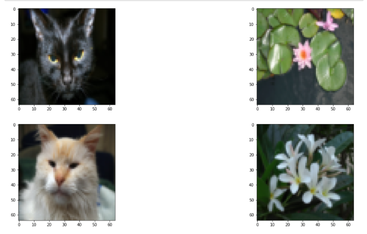
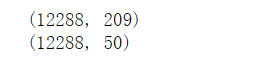
Image array processing

In order to facilitate the prediction of data later, we reconstruct the array with dimension (64, 64, 3) into an array with dimension (64x64x3, 1)

x_train_flatten = x_train.reshape(x_train.shape[0], -1).T
# Here. shape[]0] means to take the first dimension as the first dimension of the new array, and - 1 means to multiply the remaining dimensions into a new dimension
x_test_flatten = x_test.reshape(x_test.shape[0], -1).T

View new array shapes

print(x_train_flatten.shape)

print(x_test_flatten.shape)

Result:

Processing of picture data

We know that the pixel value is between 0 and 255. In order to center the later data processing, we will place the standardized data between [0, 1]

X_train = x_train_flatten / 255.0
X_test = x_test_flatten / 255.0

Gradient descent method for constructing logistic regression

sigmoid function

def sigmoid(z):
    s = 1 / (1 + np.exp(-z))
    return s

Initialize the function of w, b

def initialize_w_b(dim):
    w = np.zeros(shape=(dim,1))
    
    b = 0
    assert(w.shape == (dim, 1))
    assert(isinstance(b, float) or isinstance(b, int)) # It's OK not to write this here, but we should be more rigorous in order to standardize the code and avoid unnecessary errors
    
    return (w, b)
def initialize_w_b(dim):
    w = np.zeros(shape=(dim,1))
    
    b = 0
    assert(w.shape == (dim, 1))
    assert(isinstance(b, float) or isinstance(b, int)) # It's OK not to write this here, but we should be more rigorous in order to standardize the code and avoid unnecessary errors
    
    return (w, b)

Propagation function

def propagate(w, b, X, Y):
    
    m = X.shape[1]
    # Forward propagation
    z  = sigmoid(np.dot(w.T, X) + b)
    # cost function 
    cost = (-1) * np.sum(Y * np.log(z) + (1 - Y) * (np.log(1 - z)))
    
    # Back propagation
    dw = (1 / m) * np.dot(X, (z- Y).T)
    db = (1/ m) * np.sum(z -  Y)
    
    assert(dw.shape == w.shape)
    assert(db.dtype == float)
    cost = np.squeeze(cost) # Eliminate the value of 1 in the shape (i.e. dimension reduction)
    assert(cost.shape == ())
    # Dictionary storage dw, db
    grads = {
        'dw':dw,
        'db':db
    }
    return (grads, cost)

Optimization function

def  optimizer(w, b, X, Y, num_iterations, learning_rate,):
    costs = []
    
    for i in range (num_iterations):
        grads, cost = propagate(w, b, X, Y)
        
        dw = grads['dw']
        db = grads['db']
        # Update w, b
        w = w - learning_rate * dw
        b = b - learning_rate * db
        
        if i % 100 == 0:
            costs.append(cost) # Value of storage cost function
            print("Number of iterations: i%，Error value:%f" % (i, cost))
            
    params = {
        'w':w,
        'b':b
    }
    grads ={
        'dw':dw,
        'db':db
    }
    return (params, grads, costs)

In this way, we completed the gradient descent of simple logistic regression

Prediction function

During the prediction of the model, we may have values with tag values between (0,1). Therefore, we need to carry out the following processing

def predict(w, b, X):
    m  = X.shape[1] #Number of pictures
    Y_prediction = np.zeros((1,m)) 
    w = w.reshape(X.shape[0],1)
    
    #Calculate and predict the probability of cats appearing in the picture
    z = sigmoid(np.dot(w.T , X) + b)
    for i in range(z.shape[1]):
        #Convert the probability z [0, i] to the actual prediction p [0, i]
        if z[0,i] > 0.5: 
        	Y_prediction[0,i] = 1  
        else: 
        	Y_prediction[0,i] = 0
    #Use assertions
    assert(Y_prediction.shape == (1,m)) # Ensure y_ Shape of prediction
    return Y_prediction

We have completed all the functions we need, and finally write an integration function

Integration function

def model(X_train, Y_train, X_test, Y_test, num_iterations, learning_rate):
    w , b = initialize_w_b(X_train.shape[0])
    
    parameters , grads , costs = optimizer(w , b , X_train , Y_train,num_iterations , learning_rate)
    
    #Retrieve parameters w and b from the dictionary parameters
    w , b = parameters["w"] , parameters["b"]
    
    #Predictive test / training set
    Y_prediction_test = predict(w , b, X_test)
    Y_prediction_train = predict(w , b, X_train)
    
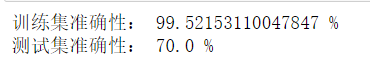
    #Print accuracy after training
    print("Training set accuracy:"  , format(100 - np.mean(np.abs(Y_prediction_train - Y_train)) * 100) ,"%")
    print("Test set accuracy:"  , format(100 - np.mean(np.abs(Y_prediction_test - Y_test)) * 100) ,"%")
    
    stored = {
            "costs" : costs,
            "Y_prediction_test" : Y_prediction_test,
            "Y_prediciton_train" : Y_prediction_train,
            "w" : w,
            "b" : b,
            "learning_rate" : learning_rate,
            "num_iterations" : num_iterations }
    return stored

model training

d = model(X_train, y_train, X_test, y_test,num_iterations=2000, learning_rate=0.01)

Result:

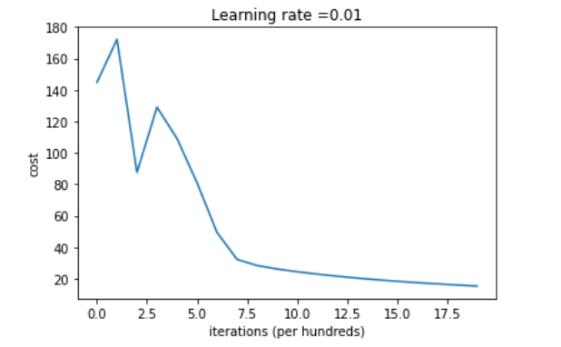
View gradient descent learning

costs = np.squeeze(d['costs'])
plt.plot(costs)
plt.ylabel('cost')
plt.xlabel('iterations ( hundreds)')
plt.title("Learning rate =" + str(d["learning_rate"]))
plt.show()

Result:

I hope this article is helpful to everyone's study!