1, MobileNetV1 network

Briefly read Google's 2017 paper mobilenets: efficient revolutionary neural networks for mobile vision applications to experience Depthwise convolution and Pointwise convolution. Also, read the code: https://github.com/OUCTheoryGroup/colab_demo/blob/master/202003_models/MobileNetV1_CIFAR10.ipynb type the code into Colab to run, observe and experience the effect.

BatchNorm2d()  : When using the nn.BatchNorm2d() layer of pytorch, it is often used to add only the number of channels (feature number) of data to be processed to the parameter. The function is to standardize the data according to the statistical mean and var, and this mena and var will be carried out in each batch (calculate the number of samples to be input for cost once. When the data set is relatively large, it will be difficult to input all samples to calculate cost once at one time, so a certain amount of samples will be input at one time for training).

Depthwise processes a three channel image using 3 × The convolution kernel of 3 is completely carried out on the two-dimensional plane. The number of convolution kernels is the same as the number of input channels, so three feature map s will be generated after operation. The parameters of convolution are: 3 × three × 3 = 27, as follows:

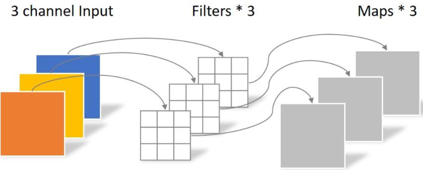
Pointwise differs in that the size of the convolution kernel is 1 × one × k. K is the number of input channels. Therefore, the convolution operation here will weight and fuse the feature maps of the previous layer. There are several feature maps with several filter s. The number of parameters is: 1 × one × three × 4 = 12, as shown in the figure below:

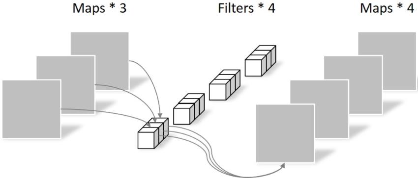
  Therefore, it can be seen that the number of parameters can be greatly reduced by using Depthwise+Pointwise to obtain four feature map s.

Code part

  MobileNet separable convolution

import torch
import torch.nn as nn
import torch.nn.functional as F
import torchvision
import torchvision.transforms as transforms
import matplotlib.pyplot as plt
import numpy as np
import torch.optim as optim

class Block(nn.Module):
    '''Depthwise conv + Pointwise conv'''
    def __init__(self, in_planes, out_planes, stride=1):
        super(Block, self).__init__()
        # Depthwise convolution, 3 * 3 convolution kernel, divided into in_planes, that is, each layer is convoluted separately
        self.conv1 = nn.Conv2d(in_planes, in_planes, kernel_size=3, stride=stride, padding=1, groups=in_planes, bias=False)
        self.bn1 = nn.BatchNorm2d(in_planes)
        # Pointwise convolution, 1 * 1 convolution kernel
        self.conv2 = nn.Conv2d(in_planes, out_planes, kernel_size=1, stride=1, padding=0, bias=False)
        self.bn2 = nn.BatchNorm2d(out_planes)

    def forward(self, x):
        out = F.relu(self.bn1(self.conv1(x)))
        out = F.relu(self.bn2(self.conv2(out)))
        return out

  Create DataLoader

# Using GPU training, you can set it in the menu "code execution tool" - > "change runtime type"
device = torch.device("cuda:0" if torch.cuda.is_available() else "cpu")

transform_train = transforms.Compose([
    transforms.RandomCrop(32, padding=4),
    transforms.RandomHorizontalFlip(),
    transforms.ToTensor(),
    transforms.Normalize((0.4914, 0.4822, 0.4465), (0.2023, 0.1994, 0.2010))])

transform_test = transforms.Compose([
    transforms.ToTensor(),
    transforms.Normalize((0.4914, 0.4822, 0.4465), (0.2023, 0.1994, 0.2010))])

trainset = torchvision.datasets.CIFAR10(root='./data', train=True,  download=True, transform=transform_train)
testset  = torchvision.datasets.CIFAR10(root='./data', train=False, download=True, transform=transform_test)

trainloader = torch.utils.data.DataLoader(trainset, batch_size=128, shuffle=True, num_workers=2)
testloader = torch.utils.data.DataLoader(testset, batch_size=128, shuffle=False, num_workers=2)

Create MobileNetV1 network

32×32×3 ==>

32×32×32 ==> 32×32×64 ==> 16×16×128 ==> 16×16×128 ==>

8×8×256 ==> 8×8×256 ==> 4×4×512 ==> 4×4×512 ==>

2×2×1024 ==> 2×2×1024

Next is the mean pooling = = > 1 × one × one thousand and twenty-four

Finally, it is fully connected to 10 output nodes

class MobileNetV1(nn.Module):
    # (128,2) means conv planes=128, stride=2
    cfg = [(64,1), (128,2), (128,1), (256,2), (256,1), (512,2), (512,1), 
           (1024,2), (1024,1)]

    def __init__(self, num_classes=10):
        super(MobileNetV1, self).__init__()
        self.conv1 = nn.Conv2d(3, 32, kernel_size=3, stride=1, padding=1, bias=False)
        self.bn1 = nn.BatchNorm2d(32)
        self.layers = self._make_layers(in_planes=32)
        self.linear = nn.Linear(1024, num_classes)

    def _make_layers(self, in_planes):
        layers = []
        for x in self.cfg:
            out_planes = x[0]
            stride = x[1]
            layers.append(Block(in_planes, out_planes, stride))
            in_planes = out_planes
        return nn.Sequential(*layers)

    def forward(self, x):
        out = F.relu(self.bn1(self.conv1(x)))
        out = self.layers(out)
        out = F.avg_pool2d(out, 2)
        out = out.view(out.size(0), -1)
        out = self.linear(out)
        return out

Instantiation network

# Put the network on the GPU
net = MobileNetV1().to(device)
criterion = nn.CrossEntropyLoss()
optimizer = optim.Adam(net.parameters(), lr=0.001)

model training

for epoch in range(10):  # Repeat multiple rounds
    for i, (inputs, labels) in enumerate(trainloader):
        inputs = inputs.to(device)
        labels = labels.to(device)
        # Optimizer gradient zeroing
        optimizer.zero_grad()
        # Forward propagation + back propagation + optimization 
        outputs = net(inputs)
        loss = criterion(outputs, labels)
        loss.backward()
        optimizer.step()
        # Output statistics
        if i % 100 == 0:   
            print('Epoch: %d Minibatch: %5d loss: %.3f' %(epoch + 1, i + 1, loss.item()))

print('Finished Training')

Model test  

correct = 0
total = 0

for data in testloader:
    images, labels = data
    images, labels = images.to(device), labels.to(device)
    outputs = net(images)
    _, predicted = torch.max(outputs.data, 1)
    total += labels.size(0)
    correct += (predicted == labels).sum().item()

print('Accuracy of the network on the 10000 test images: %.2f %%' % (
    100 * correct / total))

2, MobileNetV2 network

Briefly read Google's paper mobilenetv2: inverted residuals and linear bots on CVPR2018 to experience the improvement of the second version. Read code: https://github.com/OUCTheoryGroup/colab_demo/blob/master/202003_models/MobileNetV2_CIFAR10.ipynb type the code into Colab to run, observe and experience the effect.

The first major change of MobileNet V2: an Inverted residual block is designed

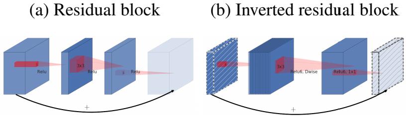
For bottleneck in ResNet, use 1x1 convolution to reduce the number of channels from 256 to 64, and then conduct 3x3 convolution, otherwise the calculation amount of intermediate 3x3 convolution is too large. So bottleneck is wide on both sides and narrow in the middle (also the origin of the name).

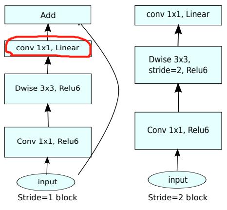
Now the 3x3 convolution in our middle can become Depthwise, with less computation, so we can have more channels. Therefore, MobileNet V2 first uses 1x1 convolution to increase the number of channels, then uses Depthwise 3x3 convolution, and then uses 1x1 convolution to reduce the dimension. The author calls it an Inverted residual block, which is wide in the middle and narrow on both sides.

The second major change of MobileNet V2: remove the ReLU6 in the output part

ReLU6 is used in MobileNet V1. ReLU6 is an ordinary ReLU, but the maximum output value is limited to 6. This is to have a good numerical resolution when the mobile terminal device float16/int8 has low precision. The output of Depthwise is relatively shallow, and the application of ReLU will cause information loss, so ReLU is removed at the end (note that there is no ReLU in the red part in the figure below).

  Code part

import torch
import torch.nn as nn
import torch.nn.functional as F
import torchvision
import torchvision.transforms as transforms
import matplotlib.pyplot as plt
import numpy as np
import torch.optim as optim

class Block(nn.Module):
    '''expand + depthwise + pointwise'''
    def __init__(self, in_planes, out_planes, expansion, stride):
        super(Block, self).__init__()
        self.stride = stride
        # Increase the number of feature map s through expansion
        planes = expansion * in_planes
        self.conv1 = nn.Conv2d(in_planes, planes, kernel_size=1, stride=1, padding=0, bias=False)
        self.bn1 = nn.BatchNorm2d(planes)
        self.conv2 = nn.Conv2d(planes, planes, kernel_size=3, stride=stride, padding=1, groups=planes, bias=False)
        self.bn2 = nn.BatchNorm2d(planes)
        self.conv3 = nn.Conv2d(planes, out_planes, kernel_size=1, stride=1, padding=0, bias=False)
        self.bn3 = nn.BatchNorm2d(out_planes)

        # When the step size is 1, if the feature map channels of in and out are different, use a convolution to change the number of channels
        if stride == 1 and in_planes != out_planes:
            self.shortcut = nn.Sequential(
                nn.Conv2d(in_planes, out_planes, kernel_size=1, stride=1, padding=0, bias=False),
                nn.BatchNorm2d(out_planes))
        # When the step size is 1, if the feature map channels of in and out are the same, the input is returned directly
        if stride == 1 and in_planes == out_planes:
            self.shortcut = nn.Sequential()

    def forward(self, x):
        out = F.relu(self.bn1(self.conv1(x)))
        out = F.relu(self.bn2(self.conv2(out)))
        out = self.bn3(self.conv3(out))
        # Step size is 1, plus shortcut operation
        if self.stride == 1:
            return out + self.shortcut(x)
        # Step size 2, direct output
        else:
            return out

Create MobileNetV2 network

Note that since CIFAR10 is 32 * 32, the network has been modified to some extent.

class MobileNetV2(nn.Module):
    # (expansion, out_planes, num_blocks, stride)
    cfg = [(1,  16, 1, 1),
           (6,  24, 2, 1), 
           (6,  32, 3, 2),
           (6,  64, 4, 2),
           (6,  96, 3, 1),
           (6, 160, 3, 2),
           (6, 320, 1, 1)]

    def __init__(self, num_classes=10):
        super(MobileNetV2, self).__init__()
        self.conv1 = nn.Conv2d(3, 32, kernel_size=3, stride=1, padding=1, bias=False)
        self.bn1 = nn.BatchNorm2d(32)
        self.layers = self._make_layers(in_planes=32)
        self.conv2 = nn.Conv2d(320, 1280, kernel_size=1, stride=1, padding=0, bias=False)
        self.bn2 = nn.BatchNorm2d(1280)
        self.linear = nn.Linear(1280, num_classes)

    def _make_layers(self, in_planes):
        layers = []
        for expansion, out_planes, num_blocks, stride in self.cfg:
            strides = [stride] + [1]*(num_blocks-1)
            for stride in strides:
                layers.append(Block(in_planes, out_planes, expansion, stride))
                in_planes = out_planes
        return nn.Sequential(*layers)

    def forward(self, x):
        out = F.relu(self.bn1(self.conv1(x)))
        out = self.layers(out)
        out = F.relu(self.bn2(self.conv2(out)))
        out = F.avg_pool2d(out, 4)
        out = out.view(out.size(0), -1)
        out = self.linear(out)
        return out

Create DataLoader

# Using GPU training, you can set it in the menu "code execution tool" - > "change runtime type"
device = torch.device("cuda:0" if torch.cuda.is_available() else "cpu")

transform_train = transforms.Compose([
    transforms.RandomCrop(32, padding=4),
    transforms.RandomHorizontalFlip(),
    transforms.ToTensor(),
    transforms.Normalize((0.4914, 0.4822, 0.4465), (0.2023, 0.1994, 0.2010))])

transform_test = transforms.Compose([
    transforms.ToTensor(),
    transforms.Normalize((0.4914, 0.4822, 0.4465), (0.2023, 0.1994, 0.2010))])

trainset = torchvision.datasets.CIFAR10(root='./data', train=True,  download=True, transform=transform_train)
testset  = torchvision.datasets.CIFAR10(root='./data', train=False, download=True, transform=transform_test)

trainloader = torch.utils.data.DataLoader(trainset, batch_size=128, shuffle=True, num_workers=2)
testloader = torch.utils.data.DataLoader(testset, batch_size=128, shuffle=False, num_workers=2)

Instantiation network

# Put the network on the GPU
net = MobileNetV2().to(device)
criterion = nn.CrossEntropyLoss()
optimizer = optim.Adam(net.parameters(), lr=0.001)

model training

for epoch in range(10):  # Repeat multiple rounds
    for i, (inputs, labels) in enumerate(trainloader):
        inputs = inputs.to(device)
        labels = labels.to(device)
        # Optimizer gradient zeroing
        optimizer.zero_grad()
        # Forward propagation + back propagation + optimization 
        outputs = net(inputs)
        loss = criterion(outputs, labels)
        loss.backward()
        optimizer.step()
        # Output statistics
        if i % 100 == 0:   
            print('Epoch: %d Minibatch: %5d loss: %.3f' %(epoch + 1, i + 1, loss.item()))

print('Finished Training')

Model test  

correct = 0
total = 0

for data in testloader:
    images, labels = data
    images, labels = images.to(device), labels.to(device)
    outputs = net(images)
    _, predicted = torch.max(outputs.data, 1)
    total += labels.size(0)
    correct += (predicted == labels).sum().item()

print('Accuracy of the network on the 10000 test images: %.2f %%' % (
    100 * correct / total))

3, HybridSN hyperspectral classification network

Read the paper HybridSN: Exploring 3-D – 2-DCNN Feature Hierarchy for Hyperspectral Image Classification and think about the difference between 3D convolution and 2D convolution. Read code: https://github.com/OUCTheoryGroup/colab_demo/blob/master/202003_models/HybridSN_GRSL2020.ipynb types the code into Colab for operation, and the network part needs to be completed by itself. Train the network and test it several times. You will find that the results of each classification are different. Please think about why? At the same time, think about the problem. If you want to further improve the classification performance of hyperspectral images, how can you improve it?

In this paper, a hybrid network is constructed to solve the problem of hyperspectral image classification. Firstly, 3D convolution is used, and then 2D convolution is used.

Three dimensional convolution part:

• conv1: (1, 30, 25, 25), 8 convolution kernels of 7x3x3 = = > (8, 24, 23, 23)
• conv2: (8, 24, 23, 23), 16 5x3x3 convolution kernels = = > (16, 20, 21, 21)
• conv3: (16, 20, 21, 21), 32 convolution kernels of 3x3x3 = = > (32, 18, 19, 19)

Next, we need to carry out two-dimensional convolution, so take the previous 32*18 reshape and get (576, 19, 19)

Two dimensional convolution: (576, 19, 19) 64 3x3 convolution kernels to obtain (64, 17, 17)

Next is a flatten operation, which becomes a vector of 18496 dimensions,

Next is the full connection layer of 256128 nodes, all of which use Dropout with a ratio of 0.4,

The final output is 16 nodes, which is the final number of classification categories.

 

Code part  

Firstly, the data is obtained and the basic function library is introduced.

! wget http://www.ehu.eus/ccwintco/uploads/6/67/Indian_pines_corrected.mat
! wget http://www.ehu.eus/ccwintco/uploads/c/c4/Indian_pines_gt.mat
! pip install spectral

import numpy as np
import matplotlib.pyplot as plt
import scipy.io as sio
from sklearn.decomposition import PCA
from sklearn.model_selection import train_test_split
from sklearn.metrics import confusion_matrix, accuracy_score, classification_report, cohen_kappa_score
import spectral
import torch
import torchvision
import torch.nn as nn
import torch.nn.functional as F
import torch.optim as optim

Define HybridSN class

class_num = 16

class HybridSN(nn.Module):
''' your code here '''

# Random input to test whether the network structure is connected
# x = torch.randn(1, 1, 30, 25, 25)
# net = HybridSN()
# y = net(x)
# print(y.shape)

Create dataset

Firstly, PCA dimensionality reduction is applied to hyperspectral data; Then create a data format that can be easily processed by keras; Then 10% of the data are randomly selected as the training set and the rest as the test set.

First, define the basic function:

# Applying PCA transform to hyperspectral data X
def applyPCA(X, numComponents):
    newX = np.reshape(X, (-1, X.shape[2]))
    pca = PCA(n_components=numComponents, whiten=True)
    newX = pca.fit_transform(newX)
    newX = np.reshape(newX, (X.shape[0], X.shape[1], numComponents))
    return newX

# When a patch is extracted around a single pixel, the edge pixels cannot be obtained. Therefore, this part of pixels is padded
def padWithZeros(X, margin=2):
    newX = np.zeros((X.shape[0] + 2 * margin, X.shape[1] + 2* margin, X.shape[2]))
    x_offset = margin
    y_offset = margin
    newX[x_offset:X.shape[0] + x_offset, y_offset:X.shape[1] + y_offset, :] = X
    return newX

# The patch is extracted around each pixel and then created into a format consistent with keras processing
def createImageCubes(X, y, windowSize=5, removeZeroLabels = True):
    # padding X
    margin = int((windowSize - 1) / 2)
    zeroPaddedX = padWithZeros(X, margin=margin)
    # split patches
    patchesData = np.zeros((X.shape[0] * X.shape[1], windowSize, windowSize, X.shape[2]))
    patchesLabels = np.zeros((X.shape[0] * X.shape[1]))
    patchIndex = 0
    for r in range(margin, zeroPaddedX.shape[0] - margin):
        for c in range(margin, zeroPaddedX.shape[1] - margin):
            patch = zeroPaddedX[r - margin:r + margin + 1, c - margin:c + margin + 1]   
            patchesData[patchIndex, :, :, :] = patch
            patchesLabels[patchIndex] = y[r-margin, c-margin]
            patchIndex = patchIndex + 1
    if removeZeroLabels:
        patchesData = patchesData[patchesLabels>0,:,:,:]
        patchesLabels = patchesLabels[patchesLabels>0]
        patchesLabels -= 1
    return patchesData, patchesLabels

def splitTrainTestSet(X, y, testRatio, randomState=345):
    X_train, X_test, y_train, y_test = train_test_split(X, y, test_size=testRatio, random_state=randomState, stratify=y)
    return X_train, X_test, y_train, y_test

To read and create a dataset:

# Feature category
class_num = 16
X = sio.loadmat('Indian_pines_corrected.mat')['indian_pines_corrected']
y = sio.loadmat('Indian_pines_gt.mat')['indian_pines_gt']

# Proportion of samples used for testing
test_ratio = 0.90
# The size of the extracted patch around each pixel
patch_size = 25
# PCA dimension reduction is used to obtain the number of principal components
pca_components = 30

print('Hyperspectral data shape: ', X.shape)
print('Label shape: ', y.shape)

print('\n... ... PCA tranformation ... ...')
X_pca = applyPCA(X, numComponents=pca_components)
print('Data shape after PCA: ', X_pca.shape)

print('\n... ... create data cubes ... ...')
X_pca, y = createImageCubes(X_pca, y, windowSize=patch_size)
print('Data cube X shape: ', X_pca.shape)
print('Data cube y shape: ', y.shape)

print('\n... ... create train & test data ... ...')
Xtrain, Xtest, ytrain, ytest = splitTrainTestSet(X_pca, y, test_ratio)
print('Xtrain shape: ', Xtrain.shape)
print('Xtest  shape: ', Xtest.shape)

# Change the shape of xtrain and ytrain to meet the requirements of keras
Xtrain = Xtrain.reshape(-1, patch_size, patch_size, pca_components, 1)
Xtest  = Xtest.reshape(-1, patch_size, patch_size, pca_components, 1)
print('before transpose: Xtrain shape: ', Xtrain.shape) 
print('before transpose: Xtest  shape: ', Xtest.shape) 

# In order to adapt to the pytorch structure, the data should be transferred
Xtrain = Xtrain.transpose(0, 4, 3, 1, 2)
Xtest  = Xtest.transpose(0, 4, 3, 1, 2)
print('after transpose: Xtrain shape: ', Xtrain.shape) 
print('after transpose: Xtest  shape: ', Xtest.shape) 


""" Training dataset"""
class TrainDS(torch.utils.data.Dataset): 
    def __init__(self):
        self.len = Xtrain.shape[0]
        self.x_data = torch.FloatTensor(Xtrain)
        self.y_data = torch.LongTensor(ytrain)        
    def __getitem__(self, index):
        # Return data and corresponding labels according to the index
        return self.x_data[index], self.y_data[index]
    def __len__(self): 
        # Returns the number of file data
        return self.len

""" Testing dataset"""
class TestDS(torch.utils.data.Dataset): 
    def __init__(self):
        self.len = Xtest.shape[0]
        self.x_data = torch.FloatTensor(Xtest)
        self.y_data = torch.LongTensor(ytest)
    def __getitem__(self, index):
        # Return data and corresponding labels according to the index
        return self.x_data[index], self.y_data[index]
    def __len__(self): 
        # Returns the number of file data
        return self.len

# Create trainloader and testloader
trainset = TrainDS()
testset  = TestDS()
train_loader = torch.utils.data.DataLoader(dataset=trainset, batch_size=128, shuffle=True, num_workers=2)
test_loader  = torch.utils.data.DataLoader(dataset=testset,  batch_size=128, shuffle=False, num_workers=2)

Start training

# Using GPU training, you can set it in the menu "code execution tool" - > "change runtime type"
device = torch.device("cuda:0" if torch.cuda.is_available() else "cpu")

# Put the network on the GPU
net = HybridSN().to(device)
criterion = nn.CrossEntropyLoss()
optimizer = optim.Adam(net.parameters(), lr=0.001)

# Start training
total_loss = 0
for epoch in range(100):
    for i, (inputs, labels) in enumerate(train_loader):
        inputs = inputs.to(device)
        labels = labels.to(device)
        # Optimizer gradient zeroing
        optimizer.zero_grad()
        # Forward propagation + back propagation + optimization 
        outputs = net(inputs)
        loss = criterion(outputs, labels)
        loss.backward()
        optimizer.step()
        total_loss += loss.item()
    print('[Epoch: %d]   [loss avg: %.4f]   [current loss: %.4f]' %(epoch + 1, total_loss/(epoch+1), loss.item()))

print('Finished Training')

Model test

count = 0
# Model test
for inputs, _ in test_loader:
    inputs = inputs.to(device)
    outputs = net(inputs)
    outputs = np.argmax(outputs.detach().cpu().numpy(), axis=1)
    if count == 0:
        y_pred_test =  outputs
        count = 1
    else:
        y_pred_test = np.concatenate( (y_pred_test, outputs) )

# Generate classification Report
classification = classification_report(ytest, y_pred_test, digits=4)
print(classification)

Spare function

The following is the standby function used to calculate the accuracy of each class and display the results for reference

from operator import truediv

def AA_andEachClassAccuracy(confusion_matrix):
    counter = confusion_matrix.shape[0]
    list_diag = np.diag(confusion_matrix)
    list_raw_sum = np.sum(confusion_matrix, axis=1)
    each_acc = np.nan_to_num(truediv(list_diag, list_raw_sum))
    average_acc = np.mean(each_acc)
    return each_acc, average_acc


def reports (test_loader, y_test, name):
    count = 0
    # Model test
    for inputs, _ in test_loader:
        inputs = inputs.to(device)
        outputs = net(inputs)
        outputs = np.argmax(outputs.detach().cpu().numpy(), axis=1)
        if count == 0:
            y_pred =  outputs
            count = 1
        else:
            y_pred = np.concatenate( (y_pred, outputs) )

    if name == 'IP':
        target_names = ['Alfalfa', 'Corn-notill', 'Corn-mintill', 'Corn'
                        ,'Grass-pasture', 'Grass-trees', 'Grass-pasture-mowed', 
                        'Hay-windrowed', 'Oats', 'Soybean-notill', 'Soybean-mintill',
                        'Soybean-clean', 'Wheat', 'Woods', 'Buildings-Grass-Trees-Drives',
                        'Stone-Steel-Towers']
    elif name == 'SA':
        target_names = ['Brocoli_green_weeds_1','Brocoli_green_weeds_2','Fallow','Fallow_rough_plow','Fallow_smooth',
                        'Stubble','Celery','Grapes_untrained','Soil_vinyard_develop','Corn_senesced_green_weeds',
                        'Lettuce_romaine_4wk','Lettuce_romaine_5wk','Lettuce_romaine_6wk','Lettuce_romaine_7wk',
                        'Vinyard_untrained','Vinyard_vertical_trellis']
    elif name == 'PU':
        target_names = ['Asphalt','Meadows','Gravel','Trees', 'Painted metal sheets','Bare Soil','Bitumen',
                        'Self-Blocking Bricks','Shadows']
    
    classification = classification_report(y_test, y_pred, target_names=target_names)
    oa = accuracy_score(y_test, y_pred)
    confusion = confusion_matrix(y_test, y_pred)
    each_acc, aa = AA_andEachClassAccuracy(confusion)
    kappa = cohen_kappa_score(y_test, y_pred)
    
    return classification, confusion, oa*100, each_acc*100, aa*100, kappa*100

The test results are written in the document:

classification, confusion, oa, each_acc, aa, kappa = reports(test_loader, ytest, 'IP')
classification = str(classification)
confusion = str(confusion)
file_name = "classification_report.txt"

with open(file_name, 'w') as x_file:
    x_file.write('\n')
    x_file.write('{} Kappa accuracy (%)'.format(kappa))
    x_file.write('\n')
    x_file.write('{} Overall accuracy (%)'.format(oa))
    x_file.write('\n')
    x_file.write('{} Average accuracy (%)'.format(aa))
    x_file.write('\n')
    x_file.write('\n')
    x_file.write('{}'.format(classification))
    x_file.write('\n')
    x_file.write('{}'.format(confusion))

The following code is used to display the classification results:

# load the original image
X = sio.loadmat('Indian_pines_corrected.mat')['indian_pines_corrected']
y = sio.loadmat('Indian_pines_gt.mat')['indian_pines_gt']

height = y.shape[0]
width = y.shape[1]

X = applyPCA(X, numComponents= pca_components)
X = padWithZeros(X, patch_size//2)

# Pixel by pixel prediction category
outputs = np.zeros((height,width))
for i in range(height):
    for j in range(width):
        if int(y[i,j]) == 0:
            continue
        else :
            image_patch = X[i:i+patch_size, j:j+patch_size, :]
            image_patch = image_patch.reshape(1,image_patch.shape[0],image_patch.shape[1], image_patch.shape[2], 1)
            X_test_image = torch.FloatTensor(image_patch.transpose(0, 4, 3, 1, 2)).to(device)                                   
            prediction = net(X_test_image)
            prediction = np.argmax(prediction.detach().cpu().numpy(), axis=1)
            outputs[i][j] = prediction+1
    if i % 20 == 0:
        print('... ... row ', i, ' handling ... ...')

predict_image = spectral.imshow(classes = outputs.astype(int),figsize =(5,5))