Catalog
2.1 introduction to data splitting
2.2 manual data splitting function
2.3 call the data splitting function in sklearn, train ﹐ test ﹐ split()
3. Indicators for evaluation of classification results
3.2 confusion matrix and its derivatives
3.3.3 comparison between PR curve and ROC curve
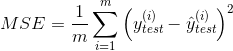
4. Indicators to evaluate regression results
4.1.2 root mean square error (RMSE)
4.1.3 mean absolute error (MAE)
1. Learning objectives
1. Data splitting: training data set and test data set
2. Evaluation and classification results: accuracy, confusion matrix, accuracy, recall, F1 score, ROC curve, etc
3. Evaluation of regression results: MSE, RMSE, MAE and R ﹐ squared
2. Data splitting
2.1 introduction to data splitting
The original data needs to be divided into two parts: training data and test data. The former is used to train the model and the latter to test the effect of the model.
If the data is randomly arranged, the original data can be cut into two parts (80% for training and 20% for testing) according to a certain proportion. If the data is arranged in a certain order, it is better to disorder the data first and then segment it. At this time, if the characteristics and labels of data are stored separately, two methods can be considered: the first is to merge them and then shuffle them; the second is to generate a shuffled index to access the corresponding data through the index [1].
2.2 manual data splitting function
import numpy as np
from sklearn import datasets

iris = datasets.load_iris()
X = iris.data
y = iris.target

def train_test_split(X, y, test_size = 0.2, random_state = None):
    if random_state != None:
        index = np.random.permutation(len(y))
    else:
        index = np.arange(len(y))
    test_len = int(test_size * len(y))
    test_index = index[:test_len]
    train_index = index[test_len:]
    X_train, y_train = X[train_index], y[train_index]
    X_test, y_test = X[test_index], y[test_index]
    return X_train, X_test, y_train, y_test

X_train, X_test, y_train, y_test = train_test_split(X, y, random_state = 2020)
print(X_train, X_test, y_train, y_test)
2.3 call the data splitting function in sklearn, train ﹐ test ﹐ split()
import numpy as np
from sklearn import datasets
from sklearn.model_selection import train_test_split

iris = datasets.load_iris()
X = iris.data
y = iris.target

X_train, X_test, y_tain, y_test = train_test_split(X, y, test_size = 0.2)
print(X_train, X_test, y_train, y_test)
3. Indicators for evaluation of classification results
3.1 accuracy
3.1.1 definition
Definition: the proportion of correctly classified samples.
Accuracy is easy to understand and widely applicable, but sometimes it is not the best index to evaluate a classification model.
3.1.2 calculation of accuracy rate by programming (taking the classification of iris data by KNN as an example)
import numpy as np
from sklearn import datasets
from sklearn.model_selection import train_test_split
from sklearn.neighbors import KNeighborsClassifier
# Import evaluation index module
from sklearn.metrics import accuracy_score

iris = datasets.load_iris()
X = iris.data
y = iris.target

X_train, X_test, y_train, y_test = train_test_split(X, y, test_size = 0.2)

knn_clf = KNeighborsClassifier(n_neighbors = 5)
knn_clf.fit(X_train, y_train)
predictions = knn_clf.predict(X_test)

# Manual calculation
accuracy_by_hands = np.sum(predictions == y_test) / len(y_test)
print(accuracy_by_hands)
# Packet calculation
accuracy_by_sklearn = accuracy_score(y_test, predictions)
print(accuracy_by_sklearn)
3.2 confusion matrix and its derivatives
3.2.1 confusion matrix
When using the accuracy to evaluate the classification algorithm, there may be a lot of problems. Especially in the case of unbalanced samples.
For example, for a cancer prediction system, the accuracy of prediction is 99.9% by inputting examination indexes to determine whether there is cancer. Is this system good or bad?
If the probability of cancer is 0.1%, there is no need for any machine learning algorithm at all. As long as the system output is healthy for all people, the accuracy can reach 99.9%. In other words, for extremely skewed data, only using classification accuracy can not measure its effect correctly.
At this point, we need to use the confusion matrix for further analysis [2].
For a biclassification problem, suppose that all problems are divided into two categories: 0 and 1. The confusion matrix is a matrix of 2 * 2
| Forecast value: 0 | Forecast value: 1 | |
| True value: 0 | TN (true Yin) | FP (false positive) |
| True value: 1 | FN (false negative) | TP (Zhenyang) |
3.2.2 precision
Definition: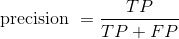 , that is, the proportion of the samples predicted as 1 that are correct.
The accuracy rate can reflect how accurate the prediction of the event we are concerned about is. Therefore, the accuracy rate is also called the precision rate.
3.2.3 recall
Definition: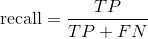 , that is, the proportion of the samples with the correct prediction in the real 1.
The recall rate reflects how likely it is to be successful in the event we are concerned about. The larger the recall rate is, the more comprehensive the sample can be covered by the successful prediction. Therefore, recall rate is also called recall rate.
For example, the recall rate of the above cancer prediction system problem is better than the accuracy rate and accuracy rate to reflect the advantages and disadvantages of the system prediction effect.
3.2.4 F1 value
There is a changing relationship between the accuracy rate and recall rate. Therefore, in this case, it is difficult to judge which classification model is better by comparing the accuracy and recall of different models at the same time. Therefore, the index of F1 value appears. The F1 value unifies the accuracy rate and recall rate into an indicator. By comparing this unified parameter, we can judge which classification model is better.
Definition: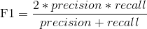 , that is, F1 value is actually the harmonic average of precision rate and recall rate.
3.2.5 accuracy
The definition of accuracy here is the same as that in 3.1. The reason why it should be put forward here is that the accuracy can also be calculated by using the confusion matrix.
According to the definition of confusion matrix and accuracy, we can get: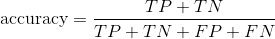
3.2.6 calculation of obfuscation matrix and its derived indexes by programming (taking the two classification of handwritten numbers by KNN as an example)
import numpy as np
from sklearn import datasets
from sklearn.model_selection import train_test_split
from sklearn.neighbors import KNeighborsClassifier
# Import evaluation index module
from sklearn.metrics import confusion_matrix
from sklearn.metrics import precision_score
from sklearn.metrics import recall_score
from sklearn.metrics import f1_score
from sklearn.metrics import accuracy_score

digits = datasets.load_digits()
X = digits.data
# Since you need to modify the label according to the original data later, it is better to pass in a copy of the array here
y = digits.target.copy()
# Structural deflection data
y[digits.target == 9] = 1
y[digits.target != 9] = 0

X_train, X_test, y_train, y_test = train_test_split(X, y, \
                                                    test_size = 0.2, \
                                                    random_state = 2019)

knn_clf = KNeighborsClassifier(n_neighbors = 5)
knn_clf.fit(X_train, y_train)
predictions = knn_clf.predict(X_test)

# Manual calculation of confusion matrix
TP = np.sum((predictions == 1) & (y_test == 1))
FP = np.sum((predictions == 1) & (y_test == 0))
TN = np.sum((predictions == 0) & (y_test == 0))
FN = np.sum((predictions == 0) & (y_test == 1))
confusion_matrix_by_hands = np.array([TN, FP, TP, FN]).reshape(2, 2)
print(confusion_matrix_by_hands)
# Confusion matrix of packet transfer calculation
print(confusion_matrix(y_test, predictions))

# Manual calculation accuracy
precision_by_hands = TP / (TP + FP)
print(precision_by_hands)
# Accuracy rate of subcontracting calculation
print(precision_score(y_test, predictions))

# Manual calculation of recall rate
recall_by_hands = TP / (TP + FN)
print(recall_by_hands)
# Calculation of recall rate by subcontracting
print(recall_score(y_test, predictions))

# Calculate F1 value manually
F1_by_hands = 2 / (1 / precision_by_hands + 1 / recall_by_hands)
print(F1_by_hands)
# Subcontracting calculation F1 value
print(f1_score(y_test, predictions))

# Manual calculation accuracy
accuracy_by_hands = (TP + TN) / (TP + TN + FP + FN)
print(accuracy_by_hands)
# Accuracy rate of subcontracting calculation
print(accuracy_score(y_test, predictions))
3.3 PR curve and ROC curve
3.3.1 PR curve
If we can sort the prediction results of the model on the samples, the more the samples in front, the more likely they will be considered as "positive examples" by the model. According to this order, the samples are regarded as positive examples one by one to predict the samples, and the corresponding accuracy rate and recall rate are obtained respectively. Taking the accuracy rate as the vertical axis and the recall rate as the horizontal axis, we can get a curve, namely PR curve [4].
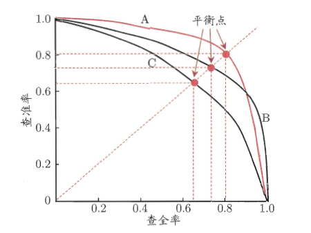 Figure 3.1 PR curve [4]
If the PR curve of one model can be completely enveloped by another, the effect of the latter is better than the former. If there is a cross, we can't judge who is better. We can only judge who is better in the specific accuracy rate and recall rate. However, people still put forward some measures to measure the pros and cons of the model with PR curve crossing. The first is to calculate the area surrounded by PR curve, the larger the area, the better the effect. But the area is not easy to calculate. So, people put forward another index, which is the equilibrium point (BEP). The equilibrium point refers to the value when the accuracy rate is equal to the recall rate. The larger the value is, the better the effect of the model is. However, the balance point is too simple. Therefore, people prefer to use F1 value instead of balance point.
3.3.2 ROC curve
It still follows the condition in PR curve, that is, the model sorts the samples according to the prediction results of the samples. The more the samples in front, the more likely they will be considered as "positive examples" by the model. The classification model is actually equivalent to finding a suitable truncation point in this sort. Different application requirements are different. If more attention is paid to the precision, the truncation point will be set in advance; if more attention is paid to the recall, the truncation point will be set later. The quality of sorting itself can directly affect the generalization ability of the model. ROC curve is proposed to study the generalization ability of the model [4] [5].
The full name of ROC curve is called "subject working characteristic" curve. Its vertical axis is the real case rate(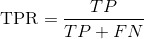 ), the horizontal axis is the false positive example rate(
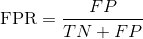 ).
).
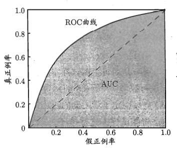 Figure 3.2 ROC curve and AUC[4]
Similar to PR curve, if the ROC curve of one model can be completely wrapped by another ROC curve, then the effect of the latter is better than the former. If there is a cross, it is impossible to determine who is better. At this time, the best way is to compare the area surrounded by ROC curve, namely AUC. The larger AUC, the better the effect of the model.
3.3.3 comparison between PR curve and ROC curve
The differences and advantages and disadvantages of the two can be referred to [6].
4. Indicators to evaluate regression results
4.1 General Indicators
4.1.1 mean square error (MSE)
4.1.2 root mean square error (RMSE)
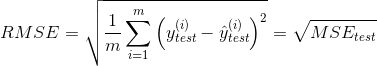
RMSE is introduced because MSE will take the square of the unit, and RMSE will eliminate the influence of the square of the unit.
4.1.3 mean absolute error (MAE)
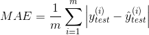
Usually, for linear regression model, its loss function is usually in the form of MSE. Because the function with absolute value is not always differentiable, it will hinder the subsequent optimization work. However, the function used to evaluate the regression model can be different from the loss function.
4.2 R^2
All of the above indicators have one common feature: they all contain units. The existence of units will lead to the comparison of models can only be limited to the data of the same unit. Sometimes we want to use a value to measure the prediction effect of different models, which is better to be a dimensionless scalar. In this way, even if the predicted data units are different, we can compare the advantages and disadvantages of the model through this dimensionless scalar [3] . And R^2 can meet this need.
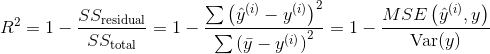
The fraction part, the denominator part refers to the error of the sample itself, and the molecule part refers to the error between the predicted result and the real value.
R^2 has the following properties:
1. R^2 is not greater than 1;
2. The closer R^2 is to 1, the better the fitting effect is;
3. If R^2 is equal to 0, the effect of the current model is equal to the benchmark model;
4. If R^2 is less than 0, the current model is not as effective as the benchmark model.
4.3 programming to realize the calculation of general index and R^2 (taking the regression prediction of linear regression to Boston house price data as an example)
import numpy as np
import matplotlib.pyplot as plt
from sklearn import datasets
from sklearn.model_selection import train_test_split
from sklearn.linear_model import LinearRegression
# Import evaluation index module
from sklearn.metrics import mean_squared_error
from sklearn.metrics import mean_absolute_error
from sklearn.metrics import r2_score

boston = datasets.load_boston()
X = boston.data[:, 5]
y = boston.target
# There is an upper limit of data, so filter out the upper limit data
X = X[y < 50.0].reshape(-1, 1)
y = y[y < 50.0].reshape(-1, 1)

X_train, X_test, y_train, y_test = train_test_split(X, y, \
                                                    test_size = 0.2, \
                                                    random_state = 2020)

lr_reg = LinearRegression()
lr_reg.fit(X_train, y_train)
predictions = lr_reg.predict(X_test)

plt.scatter(X_test, y_test, c = 'b')
plt.scatter(X_test, predictions, c = 'r')
plt.show()

# Calculate MSE manually
mse_by_hands = (np.linalg.norm(y_test - predictions, ord = 2)) **2 / len(y_test)
print(mse_by_hands)
# Subcontracting calculation MSE
print(mean_squared_error(y_test, predictions))

# Calculate RMSE manually
rmse_by_hands = (np.linalg.norm(y_test - predictions, ord = 2)) / np.sqrt(len(y_test))
print(rmse_by_hands)
# Subcontracting calculation RMSE
print(np.sqrt(mean_squared_error(y_test, predictions)))

# Manual calculation of MAE
mae_by_hands = (np.linalg.norm(y_test - predictions, ord = 1)) / len(y_test)
print(mae_by_hands)
# Subcontracting calculation MAE
print(mean_absolute_error(y_test, predictions))

# Calculate R^2 manually
r_2 = 1 - mse_by_hands / np.var(y_test)
print(r_2)
# Subcontracting calculation R^2
print(r2_score(y_test, predictions))
5. References
1. https://mp.weixin.qq.com/s/vvCM0vWH5kmRfrRWxqXT8Q
2. https://mp.weixin.qq.com/s/Fi13jaEkM5EGjmS7Mm_Bjw
3. https://mp.weixin.qq.com/s/BEmMdQd2y1hMu9wT8QYCPg
4. Chapter II of machine learning (Zhou Zhihua)
5. https://www.jianshu.com/p/c61ae11cc5f6
6. https://blog.csdn.net/weixin_31866177/article/details/88776718

