1, Decision tree

• Decision Tree (Decision Tree) is a decision analysis method that calculates the probability that the expected value of net present value is greater than or equal to zero by forming a Decision Tree on the basis of knowing the occurrence probability of various situations, evaluates the project risk and judges its feasibility. It is a graphical method of intuitively using probability analysis. Because this decision branch is drawn in a graph, it is very similar to the branch of a tree, so it is called Decision Tree In learning, the Decision Tree is a prediction model, which represents a mapping relationship between object attributes and object values. Entropy = the disorder degree of the system. The spanning tree algorithm uses entropy using algorithms ID3, C4.5 and C5.0. This measurement is based on the concept of entropy in informatics theory.
• Decision tree is a tree structure, in which each internal node represents a test on an attribute, each branch represents a test output, and each leaf node represents a category.
• Classification tree (decision tree) It is a very common classification method. It is a kind of supervised learning. The so-called supervised learning is that given a pile of samples, each sample has a set of attributes and a category. These categories are determined in advance, then a classifier can be obtained through learning, which can give correct classification to new objects. Such machine learning is called supervised learning .

advantage:

• The decision tree is easy to understand and realize. People do not need users to know a lot of background knowledge in the learning process. At the same time, it can directly reflect the characteristics of data. As long as it is explained, it has the ability to understand the meaning expressed by the decision tree.
• For the decision tree, the preparation of data is often simple or unnecessary, and it can deal with data and conventional attributes at the same time, and can make feasible and effective results for large data sources in a relatively short time.
• It is easy to evaluate the model through static test and measure the reliability of the model; if an observed model is given, it is easy to deduce the corresponding logical expression according to the generated decision tree.

Disadvantages:

• Fields of continuity are difficult to predict.
• For data with time sequence, a lot of preprocessing work is required.
• When there are too many categories, errors may increase faster.
• When the general algorithm classifies, it only classifies according to one field.

2, Related concepts

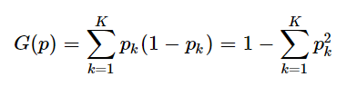
2.1 Gini index

• Gini index (Gini impure) represents the probability that a randomly selected sample in the sample set is misdivided.
• Note: the smaller the Gini index, the smaller the probability that the selected samples in the set are mixed up, that is, the higher the purity of the set, on the contrary, the more impure the set. When all samples in the set are one class, the Gini index is 0
• The Gini index is calculated as follows:
  

2.2 information entropy

• The so-called information entropy is a quite abstract concept in mathematics. Here, it is advisable to understand information entropy as the occurrence probability of a specific information. Information entropy and thermodynamic entropy are closely related. According to Charles H. Bennett's reinterpretation of Maxwell's Demon, the destruction of information is an irreversible process, so the destruction of information conforms to the second law of thermodynamics Generating information is the process of introducing negative (thermodynamic) entropy into the system, so the symbol of information entropy should be opposite to thermodynamic entropy.
• Generally speaking, when a kind of information has a higher probability of occurrence, it indicates that it is more widely spread, or more cited. We can think that from the perspective of information dissemination, information entropy can represent the value of information. In this way, we have a standard to measure the value of information and can make more inferences about the problem of knowledge circulation.
• Calculation formula:
  
• Where, X represents random variables, and the corresponding set is the set of all possible outputs, which is defined as a symbolic set. The output of random variables is represented by X. P(x) represents the output probability function. The greater the uncertainty of variables, the greater the entropy, and the greater the amount of information needed to make it clear

3, ID3 algorithm

3.1 concept

• ID3 algorithm was first proposed by J. Ross Quinlan at the University of Sydney in 1975. The core of the algorithm is "information entropy" By calculating the information gain of each attribute, ID3 algorithm considers that the attribute with high information gain is a good attribute. Each division selects the attribute with the highest information gain as the division standard, and repeats this process until a decision tree that can perfectly classify training samples is generated.

3.2 steps

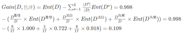
• step1: calculate the initial information entropy and use the above formula to calculate the information entropy
• Step 2: calculate the information entropy of each feature. The calculation method is to first calculate the information entropy of each feature value according to the above formula, multiply it by the proportion of the feature value, add it is the entropy of the feature, and then subtract the information entropy calculated from the win, which is the information gain. The following figure takes color as an example
• step3: sort by information gain
• step4: select the feature of maximum information gain and take this feature as the dividing node
• step5: delete the feature from the feature list, return to step 4 and continue to divide until there is no feature

3.3 code implementation

• Import package

import numpy as np
import pandas as pd
import math
import collections

• Import data

def import_data():
    data = pd.read_csv('..\\source\\watermalon.txt')
    data.head(10)
    data=np.array(data).tolist()
    # Characteristic value list
    labels = ['color and lustre', 'Root', 'Knock', 'texture', 'Umbilicus', 'Tactile sensation']

    # All possible cases corresponding to the feature
    labels_full = {}

    for i in range(len(labels)):
        labelList = [example[i] for example in data]
        uniqueLabel = set(labelList)
        labels_full[labels[i]] = uniqueLabel
    return data,labels,labels_full

• Call function to get data

data,labels,labels_full=import_data()

• Calculate the initial information entropy, that is, the information entropy before classification

def calcShannonEnt(dataSet):
    """
    Calculate the information entropy of a given data set(Shannon entropy)
    :param dataSet:
    :return:
    """
    # Calculate the total number of data sets
    numEntries = len(dataSet)

    # Used to count tags
    labelCounts = collections.defaultdict(int)

    # Loop the whole data set to get the classification label of the data
    for featVec in dataSet:
        # Get the current label
        currentLabel = featVec[-1]

        # # If the current tag is no longer in the tag set, add it (in the book)
        # if currentLabel not in labelCounts.keys():
        #     labelCounts[currentLabel] = 0
        #
        # # The number of corresponding tags in the tag set plus one
        # labelCounts[currentLabel] += 1

        # It can also be written as follows
        labelCounts[currentLabel] += 1

    # Default information entropy
    shannonEnt = 0.0

    for key in labelCounts:
        # Calculate the proportion of the current category label in the total label
        prob = float(labelCounts[key]) / numEntries

        # Find logarithm based on 2
        shannonEnt -= prob * math.log2(prob)

    return shannonEnt

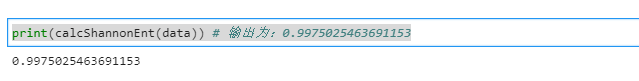
• View initial information entropy

print(calcShannonEnt(data)) # Output: 0.99750254631653

• Obtain the number of each eigenvalue, which is to prepare for the later calculation of information gain

def splitDataSet(dataSet, axis, value):
    """
    Divide the data set according to the given eigenvalue
    :param dataSet: data set
    :param axis: Coordinates of a given eigenvalue
    :param value: If a given eigenvalue satisfies the condition, only the given eigenvalue is equal to this value Will return when
    :return:
    """
    # Create a new list to prevent modifications to the original list
    retDataSet = []

    # Traverse the entire dataset
    for featVec in dataSet:
        # If the given eigenvalue is equal to the desired eigenvalue
        if featVec[axis] == value:
            # Save the contents in front of the characteristic value
            reducedFeatVec = featVec[:axis]
            # Save the content after the eigenvalue, so the given eigenvalue is removed
            reducedFeatVec.extend(featVec[axis + 1:])
            # Add to return list
            retDataSet.append(reducedFeatVec)

    return retDataSet

• Calculate the information gain to determine the best data set partition

def chooseBestFeatureToSplit(dataSet, labels):
    """
    The best data set partition feature is selected and calculated according to the information gain value
    :param dataSet:
    :return:
    """
    # Get the total number of eigenvalues of the data
    numFeatures = len(dataSet[0]) - 1

    # Calculate the basic information entropy
    baseEntropy = calcShannonEnt(dataSet)

    # The gain of basic information is 0.0
    bestInfoGain = 0.0

    # Best eigenvalue
    bestFeature = -1

    # Calculate the information entropy of each eigenvalue
    for i in range(numFeatures):
        # Get a list of all current eigenvalues in the dataset
        featList = [example[i] for example in dataSet]

        # Make the current feature unique, that is, how many kinds of current feature values are there
        uniqueVals = set(featList)

        # The new entropy represents the entropy of the current eigenvalue
        newEntropy = 0.0

        # Possibility of traversing existing features
        for value in uniqueVals:
            # At the current feature position of all data sets, find the set whose feature value is equal to the current value
            subDataSet = splitDataSet(dataSet=dataSet, axis=i, value=value)

            # Calculate the weight
            prob = len(subDataSet) / float(len(dataSet))

            # Calculate the entropy of the current eigenvalue
            newEntropy += prob * calcShannonEnt(subDataSet)

        # Calculate the "information gain"
        infoGain = baseEntropy - newEntropy

        #print('current characteristic value: '+ labels[i] +', corresponding information gain value: '+ str(infoGain)+"i equals" + str(i))

        #If the current information gain is greater than the original
        if infoGain > bestInfoGain:
            # Best information gain
            bestInfoGain = infoGain
            # The new best eigenvalue is used to divide
            bestFeature = i

    #print('features with maximum information gain: '+ labels[bestFeature])
    return bestFeature

• Judge whether the attributes of each sample set are consistent

def judgeEqualLabels(dataSet):
    """
    Judge whether each attribute set of the data set is completely consistent
    :param dataSet:
    :return:
    """
    # Calculate the total number of attributes in the sample set, and the last one is category
    feature_leng = len(dataSet[0]) - 1

    # Calculate the total number of data
    data_leng = len(dataSet)

    # Tag what is the first attribute value in each attribute
    first_feature = ''

    # Are all attribute sets completely consistent
    is_equal = True

    # Traverse all attributes
    for i in range(feature_leng):
        # Get the i-th attribute of the first sample
        first_feature = dataSet[0][i]

        # Compare with all the data in the sample set to see if the attribute is consistent
        for _ in range(1, data_leng):
            # If inequality is found, False is returned directly
            if first_feature != dataSet[_][i]:
                return False

    return is_equal

• Draw decision tree (Dictionary)

def createTree(dataSet, labels):
    """
    Create decision tree
    :param dataSet: data set
    :param labels: Feature label
    :return:
    """
    # Get the classification labels of all data sets
    classList = [example[-1] for example in dataSet]

    # Count the number of occurrences of the first label and compare it with the total number of labels. If it is equal, it means that all labels in the current list are one kind of labels. At this time, the division is stopped
    if classList.count(classList[0]) == len(classList):
        return classList[0]

    # Calculate the number of data in the first row. If there is only one, it means that all feature attributes have been traversed. The remaining one is the category label, or all samples are consistent in all attributes
    if len(dataSet[0]) == 1 or judgeEqualLabels(dataSet):
        # Returns the one that appears more frequently in the remaining tags
        return majorityCnt(classList)

    # Select the best partition feature and get the subscript of the feature
    bestFeat = chooseBestFeatureToSplit(dataSet=dataSet, labels=labels)
    print(bestFeat)
    # Get the name of the best feature
    bestFeatLabel = labels[bestFeat]
    print(bestFeatLabel)
    # A dictionary is used to store the tree structure, and the bifurcation is the divided feature name
    myTree = {bestFeatLabel: {}}

    # Delete the characteristic value of this division from the list
    del(labels[bestFeat])

    # Get all possible values of the current feature label
    featValues = [example[bestFeat] for example in dataSet]

    # Uniqueness, removing duplicate eigenvalues
    uniqueVals = set(featValues)

    # Traverse all eigenvalues
    for value in uniqueVals:
        # Get the remaining feature tags
        subLabels = labels[:]
        subTree = createTree(splitDataSet(dataSet=dataSet, axis=bestFeat, value=value), subLabels)
        # Recursive call divides all data in the data set whose feature is equal to the current feature value into the current node. During recursive call, the current feature needs to be removed first
        myTree[bestFeatLabel][value] = subTree
    return myTree

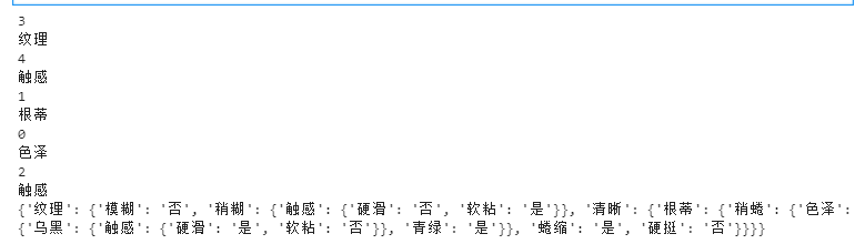
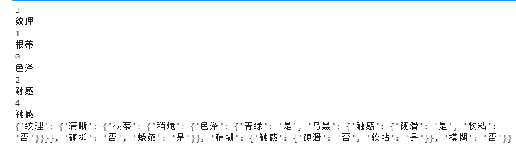
• Call the function and print, and you can see a dictionary type tree

mytree=createTree(data,labels)
print(mytree)

• Draw visual tree

import matplotlib.pylab as plt
import matplotlib

# Can display Chinese
matplotlib.rcParams['font.sans-serif'] = ['SimHei']
matplotlib.rcParams['font.serif'] = ['SimHei']

# Bifurcation node, that is, decision node
decisionNode = dict(boxstyle="sawtooth", fc="0.8")

# Leaf node
leafNode = dict(boxstyle="round4", fc="0.8")

# Arrow style
arrow_args = dict(arrowstyle="<-")


def plotNode(nodeTxt, centerPt, parentPt, nodeType):
    """
    Draw a node
    :param nodeTxt: Text information describing the node
    :param centerPt: Coordinates of text
    :param parentPt: The coordinates of the point, which also refers to the coordinates of the parent node
    :param nodeType: Node type,It is divided into leaf node and decision node
    :return:
    """
    createPlot.ax1.annotate(nodeTxt, xy=parentPt, xycoords='axes fraction',
                            xytext=centerPt, textcoords='axes fraction',
                            va="center", ha="center", bbox=nodeType, arrowprops=arrow_args)


def getNumLeafs(myTree):
    """
    Gets the number of leaf nodes
    :param myTree:
    :return:
    """
    # Count the total number of leaf nodes
    numLeafs = 0

    # Get the current first key, that is, the root node
    firstStr = list(myTree.keys())[0]

    # Get the content corresponding to the first key
    secondDict = myTree[firstStr]

    # Recursively traversing leaf nodes
    for key in secondDict.keys():
        # If the key corresponds to a dictionary, it is called recursively
        if type(secondDict[key]).__name__ == 'dict':
            numLeafs += getNumLeafs(secondDict[key])
        # If not, it means that it is a leaf node at this time
        else:
            numLeafs += 1
    return numLeafs


def getTreeDepth(myTree):
    """
    Number of depth layers obtained
    :param myTree:
    :return:
    """
    # Used to save the maximum number of layers
    maxDepth = 0

    # Get root node
    firstStr = list(myTree.keys())[0]

    # Get the content corresponding to the key
    secondDic = myTree[firstStr]

    # Traverse all child nodes
    for key in secondDic.keys():
        # If the node is a dictionary, it is called recursively
        if type(secondDic[key]).__name__ == 'dict':
            # Depth of child node plus 1
            thisDepth = 1 + getTreeDepth(secondDic[key])

        # This indicates that this is a leaf node
        else:
            thisDepth = 1

        # Replace maximum layers
        if thisDepth > maxDepth:
            maxDepth = thisDepth

    return maxDepth


def plotMidText(cntrPt, parentPt, txtString):
    """
    Calculate the middle position between the parent node and the child node, and fill in the information
    :param cntrPt: Child node coordinates
    :param parentPt: Parent node coordinates
    :param txtString: Filled text information
    :return:
    """
    # Calculate the middle position of the x-axis
    xMid = (parentPt[0]-cntrPt[0])/2.0 + cntrPt[0]
    # Calculate the middle position of the y-axis
    yMid = (parentPt[1]-cntrPt[1])/2.0 + cntrPt[1]
    # Draw
    createPlot.ax1.text(xMid, yMid, txtString)


def plotTree(myTree, parentPt, nodeTxt):
    """
    Draw all nodes of the tree and draw recursively
    :param myTree: tree
    :param parentPt: Coordinates of the parent node
    :param nodeTxt: Text information of the node
    :return:
    """
    # Calculate the number of leaf nodes
    numLeafs = getNumLeafs(myTree=myTree)

    # Calculate the depth of the tree
    depth = getTreeDepth(myTree=myTree)

    # Get the information content of the root node
    firstStr = list(myTree.keys())[0]

    # Calculate the middle coordinates of the current root node in all child nodes, that is, the offset of the current X-axis plus the calculated center position of the root node as the x-axis (for example, the first time: the initial x-offset is: - 1/2W, the calculated center position of the root node is: (1+W)/2W, add to get: 1 / 2), and the current Y-axis offset is the y-axis
    cntrPt = (plotTree.xOff + (1.0 + float(numLeafs))/2.0/plotTree.totalW, plotTree.yOff)

    # Draw the connection between the node and the parent node
    plotMidText(cntrPt, parentPt, nodeTxt)

    # Draw the node
    plotNode(firstStr, cntrPt, parentPt, decisionNode)

    # Get the subtree corresponding to the current root node
    secondDict = myTree[firstStr]

    # Calculate the new y-axis offset and move down 1/D, that is, the drawing y-axis of the next layer
    plotTree.yOff = plotTree.yOff - 1.0/plotTree.totalD

    # Loop through all key s
    for key in secondDict.keys():
        # If the current key is a dictionary and there are subtrees, it will be traversed recursively
        if isinstance(secondDict[key], dict):
            plotTree(secondDict[key], cntrPt, str(key))
        else:
            # Calculate the new X-axis offset, that is, the x-axis coordinate drawn by the next leaf moves 1/W to the right
            plotTree.xOff = plotTree.xOff + 1.0/plotTree.totalW
            # Open the annotation to observe the coordinate changes of leaf nodes
            # print((plotTree.xOff, plotTree.yOff), secondDict[key])
            # Draw leaf node
            plotNode(secondDict[key], (plotTree.xOff, plotTree.yOff), cntrPt, leafNode)
            # Draw the content of the middle line between the leaf node and the parent node
            plotMidText((plotTree.xOff, plotTree.yOff), cntrPt, str(key))

    # Before returning to recursion, you need to increase the offset of the y-axis and move it up by 1/D, that is, return to draw the y-axis of the previous layer
    plotTree.yOff = plotTree.yOff + 1.0/plotTree.totalD


def createPlot(inTree):
    """
    Decision tree to be drawn
    :param inTree: Decision tree dictionary
    :return:
    """
    # Create an image
    fig = plt.figure(1, facecolor='white')
    fig.clf()
    axprops = dict(xticks=[], yticks=[])
    createPlot.ax1 = plt.subplot(111, frameon=False, **axprops)
    # Calculate the total width of the decision tree
    plotTree.totalW = float(getNumLeafs(inTree))
    # Calculate the total depth of the decision tree
    plotTree.totalD = float(getTreeDepth(inTree))
    # The initial x-axis offset, that is - 1/2W, moves 1/W to the right each time, that is, the x coordinates drawn by the first leaf node are: 1/2W, the second: 3/2W, the third: 5/2W, and the last: (W-1)/2W
    plotTree.xOff = -0.5/plotTree.totalW
    # The initial y-axis offset, moving down or up 1/D each time
    plotTree.yOff = 1.0
    # Call the function to draw the node image
    plotTree(inTree, (0.5, 1.0), '')
    # draw
    plt.show()


if __name__ == '__main__':
    createPlot(mytree)

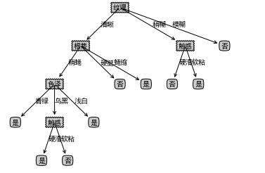
• give the result as follows
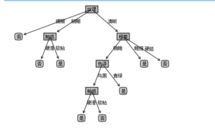
• There are some labels missing from the tree. You need to complete the tree and output it again

def makeTreeFull(myTree, labels_full, default):
    """
    Complete the nonexistent feature labels in the tree to the category with the most occurrences in the parent node
    :param myTree: Generated tree
    :param labels_full: All labels for the feature
    :param parentClass: Maximum categories in parent node
    :param default: If the parent node in the missing label cannot judge the category, this value is used
    :return:
    """
    # The parent node mentioned here is the current root node, and the feature label that does not exist under the current root node is taken as the child node

    # Get the current root node
    root_key = list(myTree.keys())[0]

    # Get all the classifications under the root node, which may be child nodes (good melon or bad melon) or not child nodes (attribute values divided again)
    sub_tree = myTree[root_key]

    # If it is a leaf node, it ends
    if isinstance(sub_tree, str):
        return

    # Find the category that uses the most under the current node classification, and use the classification result as the classification of the new feature label. For example, if there is no light white under the color, use the cyan classification in the color as the light white classification
    root_class = []
    # Record the classified results
    for sub_key in sub_tree.keys():
        if isinstance(sub_tree[sub_key], str):
            root_class.append(sub_tree[sub_key])

    # Find the category that appears most in this layer, and the same situation may occur. Take one
    if len(root_class):
        most_class = collections.Counter(root_class).most_common(1)[0][0]
    else:
        most_class = None# There are no classified attributes under the current node
    # print(most_class)

    # Loop through all feature labels and add non-existent labels
    for label in labels_full[root_key]:
        if label not in sub_tree.keys():
            if most_class is not None:
                sub_tree[label] = most_class
            else:
                sub_tree[label] = default

    # Recursive processing
    for sub_key in sub_tree.keys():
        if isinstance(sub_tree[sub_key], dict):
            makeTreeFull(myTree=sub_tree[sub_key], labels_full=labels_full, default=default)

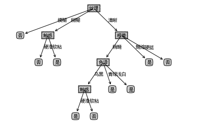
• Call and draw the tree again

makeTreeFull(mytree,labels_full,default='unknown')
createPlot(mytree)

• Implementing ID3 using sklearn

# Import package
import pandas as pd
from sklearn import tree
import graphviz

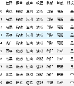
• Read the file and you can see the read data

df = pd.read_csv('..\\source\\watermalon.txt')
df.head(10)

• Convert all eigenvalues to numbers

df['color and lustre']=df['color and lustre'].map({'plain ':1,'dark green':2,'Black':3})
df['Root']=df['Root'].map({'Slightly curled':1,'Curl up':2,'Stiff':3})
df['stroke ']=df['stroke '].map({'Crisp':1,'Turbid sound':2,'Dull':3})
df['texture']=df['texture'].map({'clear':1,'Slightly paste':2,'vague':3})
df['Umbilicus']=df['Umbilicus'].map({'flat':1,'Slightly concave':2,'sunken':3})
df['Tactile sensation'] = np.where(df['Tactile sensation']=="Hard slip",1,2)
df['Good melon'] = np.where(df['Good melon']=="yes",1,0)
x_train=df[['color and lustre','Root','stroke ','texture','Umbilicus','Tactile sensation']]
y_train=df['Good melon']
print(df)
id3=tree.DecisionTreeClassifier(criterion='entropy')
id3=id3.fit(x_train,y_train)
print(id3)

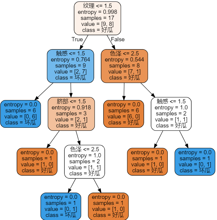
• Get the following pictures
  
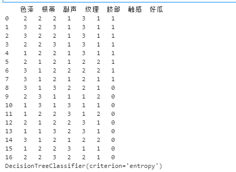
• Training and visualization. The parameter of DecisionTreeClassifier is entropy id3 algorithm. The default is CART algorithm, and there is no C4.5 algorithm

id3=tree.DecisionTreeClassifier(criterion='entropy')
id3=id3.fit(x_train,y_train)
labels = ['color and lustre', 'Root', 'Knock', 'texture', 'Umbilicus', 'Tactile sensation']
dot_data = tree.export_graphviz(id3
,feature_names=labels
,class_names=["Good melon","Bad melon"]
,filled=True
,rounded=True
)
graph = graphviz.Source(dot_data)
graph

4, C4.5 algorithm

4.1 introduction

• C4.5 is a decision tree algorithm, which is an improved algorithm of the core algorithm ID3 of the decision tree (the decision tree is the organization of decision-making nodes like a tree, which is actually an inverted tree)

4.2 steps

• As mentioned above, the core of C4.5 algorithm is still ID3, so the steps are the same, except that the information gain is changed into the information gain rate, that is, the information gain is calculated and then divided by the information entropy of the feature

4.3 change code

• Because it becomes less, we just add another step to get the information gain to get the information gain rate

## Implement C4.5 algorithm
def chooseBestFeatureToSplit_4(dataSet, labels):
    """
    The best data set partition feature is selected and calculated according to the information gain value
    :param dataSet:
    :return:
    """
    # Get the total number of eigenvalues of the data
    numFeatures = len(dataSet[0]) - 1

    # Calculate the basic information entropy
    baseEntropy = calcShannonEnt(dataSet)

    # The gain of basic information is 0.0
    bestInfoGain = 0.0

    # Best eigenvalue
    bestFeature = -1

    # Calculate the information entropy of each eigenvalue
    for i in range(numFeatures):
        # Get a list of all current eigenvalues in the dataset
        featList = [example[i] for example in dataSet]

        # Make the current feature unique, that is, how many kinds of current feature values are there
        uniqueVals = set(featList)

        # The new entropy represents the entropy of the current eigenvalue
        newEntropy = 0.0

        # Possibility of traversing existing features
        for value in uniqueVals:
            # At the current feature position of all data sets, find the set whose feature value is equal to the current value
            subDataSet = splitDataSet(dataSet=dataSet, axis=i, value=value)

            # Calculate the weight
            prob = len(subDataSet) / float(len(dataSet))

            # Calculate the entropy of the current eigenvalue
            newEntropy += prob * calcShannonEnt(subDataSet)

        # Calculate the "information gain"
        infoGain = baseEntropy - newEntropy
        infoGain = infoGain/newEntropy

        #print('current characteristic value: '+ labels[i] +', corresponding information gain value: '+ str(infoGain)+"i equals" + str(i))

        #If the current information gain is greater than the original
        if infoGain > bestInfoGain:
            # Best information gain
            bestInfoGain = infoGain
            # The new best eigenvalue is used to divide
            bestFeature = i

    #print('features with maximum information gain: '+ labels[bestFeature])
    return bestFeature

• I still changed the function of creating the tree to avoid confusion

def createTree_4(dataSet, labels):
    """
    Create decision tree
    :param dataSet: data set
    :param labels: Feature label
    :return:
    """
    # Get the classification labels of all data sets
    classList = [example[-1] for example in dataSet]

    # Count the number of occurrences of the first label and compare it with the total number of labels. If it is equal, it means that all labels in the current list are one kind of labels. At this time, the division is stopped
    if classList.count(classList[0]) == len(classList):
        return classList[0]

    # Calculate the number of data in the first row. If there is only one, it means that all feature attributes have been traversed. The remaining one is the category label, or all samples are consistent in all attributes
    if len(dataSet[0]) == 1 or judgeEqualLabels(dataSet):
        # Returns the one that appears more frequently in the remaining tags
        return majorityCnt(classList)

    # Select the best partition feature and get the subscript of the feature
    bestFeat = chooseBestFeatureToSplit_4(dataSet=dataSet, labels=labels)
    print(bestFeat)
    # Get the name of the best feature
    bestFeatLabel = labels[bestFeat]
    print(bestFeatLabel)
    # A dictionary is used to store the tree structure, and the bifurcation is the divided feature name
    myTree = {bestFeatLabel: {}}

    # Delete the characteristic value of this division from the list
    del(labels[bestFeat])

    # Get all possible values of the current feature label
    featValues = [example[bestFeat] for example in dataSet]

    # Uniqueness, removing duplicate eigenvalues
    uniqueVals = set(featValues)

    # Traverse all eigenvalues
    for value in uniqueVals:
        # Get the remaining feature tags
        subLabels = labels[:]
        subTree = createTree(splitDataSet(dataSet=dataSet, axis=bestFeat, value=value), subLabels)
        # Recursive call divides all data in the data set whose feature is equal to the current feature value into the current node. During recursive call, the current feature needs to be removed first
        myTree[bestFeatLabel][value] = subTree
    return myTree

• Call the function and look at the dictionary tree

mytree_4=createTree_4(data,labels)
print(mytree_4)

• Then complete it and then visualize it

makeTreeFull(mytree_4,labels_full,default='unknown')
createPlot(mytree_4)

5, CART algorithm

5.1 introduction

CART algorithm is a binary recursive segmentation technology, which divides the current sample into two sub samples, so that each non leaf node has two branches. Therefore, the decision tree generated by CART algorithm is a binary tree with simple structure. Because CART algorithm is a binary tree, it can only be "yes" or "no" in each step of decision-making. Even if a feature has multiple values, it also divides the data into two parts. The CART algorithm is mainly divided into two steps

(1) Recursive partition of samples for tree building process

(2) Pruning with validation data

5.2 steps

• step1: select an independent variable, and then select a value to divide the dimensional space into two parts. All points of one part are satisfied, and all points of the other part are satisfied. For discontinuous variables, there are only two values of attribute value, that is, equal to or not equal to the value.

• Step 2: recursive processing. Select a new attribute from the above two parts according to step 1 and continue to divide until the whole dimensional space is divided. There is a problem in the division. What criteria is it divided according to? For a variable attribute, its partition point is the midpoint of a pair of continuous variable attribute values. Assuming that an attribute of a set of samples has a continuous value, there will be a split point, and each split point is the mean of two adjacent continuous values. The division of each attribute is sorted according to the amount of impurities that can be reduced, and the reduction of impurities is defined as the sum of the impurities before division minus the proportion of impurity mass division of each node after division. The Gini index is commonly used in impurity measurement methods. Assuming that a sample has a common class, the Gini impurity of a node can be defined as

• Where Pi represents the probability of belonging to class i. When Gini(A)=0, all samples belong to the same class. When all classes appear in the node with equal probability, Gini(A) is maximized. At this time, Pi has the above theoretical basis. The actual recursive partition process is as follows: if all samples of the current node do not belong to the same class or only one sample is left, then this node is a non leaf node, Therefore, each attribute of the sample and the corresponding splitting point of each attribute will be tried to find the partition with the largest impurity variable, and the subtree divided by this attribute is the optimal branch.

5.3 implementation using sklearn Library

• Import package

import pandas as pd
from sklearn import tree
import graphviz

• Import data and read

df = pd.read_csv('..\\source\\watermalon.txt')
df.head(10)

• Convert eigenvalues to numbers

df['color and lustre']=df['color and lustre'].map({'plain ':1,'dark green':2,'Black':3})
df['Root']=df['Root'].map({'Slightly curled':1,'Curl up':2,'Stiff':3})
df['stroke ']=df['stroke '].map({'Crisp':1,'Turbid sound':2,'Dull':3})
df['texture']=df['texture'].map({'clear':1,'Slightly paste':2,'vague':3})
df['Umbilicus']=df['Umbilicus'].map({'flat':1,'Slightly concave':2,'sunken':3})
df['Tactile sensation'] = np.where(df['Tactile sensation']=="Hard slip",1,2)
df['Good melon'] = np.where(df['Good melon']=="yes",1,0)
x_train=df[['color and lustre','Root','stroke ','texture','Umbilicus','Tactile sensation']]
y_train=df['Good melon']

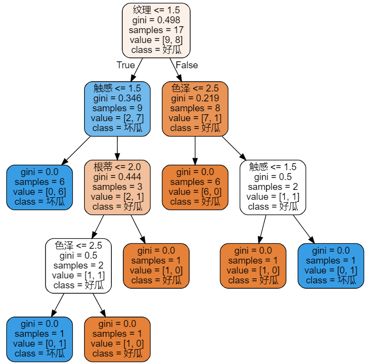
• Train the tree and visualize it

# Build models and train
gini=tree.DecisionTreeClassifier()
gini=gini.fit(x_train,y_train)
#Visualization of decision tree
gini_data = tree.export_graphviz(gini
,feature_names=labels
,class_names=["Good melon","Bad melon"]
,filled=True
,rounded=True
)
gini_graph = graphviz.Source(gini_data)
gini_graph

6, Summary

It is not difficult to understand the decision tree, that is, it is necessary to know the division basis of each algorithm. The steps are roughly to calculate the evaluation criteria first, then sort according to the evaluation results, and finally recursively build the tree according to the order.

7, Reference

Decision tree
Information entropy
CART algorithm
Gini Gini index
Implementation of ID3 decision tree in watermelon book