Chapter IV decision tree

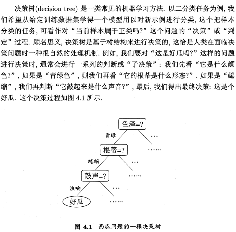
1 basic process

2 division selection

With the continuous division process, we hope that the samples contained in the branch nodes of the decision tree belong to the same category as much as possible, that is, the "purity" of the nodes is getting higher and higher.

2.1 information gain

2.1.1 what is information entropy

https://www.zhihu.com/question/22178202

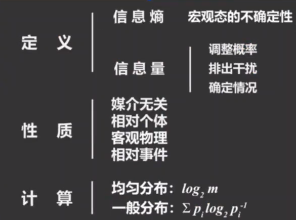
What is entropy: the uncertainty of a thing.

Information: something that eliminates uncertainty.

Function of information: adjust probability; Eliminate interference; Determine the situation (for example, the melon seller said that it is cooked and sweet).

Noise: something that cannot eliminate someone's uncertainty about something.

Data = information + noise

2.1.2 how to quantify entropy - equal probability

Refer to an uncertain event as a unit. For example, a coin toss is recorded as 1bit.

For example, eight uncertain cases with equal probability are equivalent to tossing coins three times, that is, 2 ^ 3 possible cases, and the entropy is 3bit.

For example, 10 uncertain cases with equal probability are equivalent to tossing log10 coins, that is, 2^log10 possible cases. The entropy is log10bit, and the logarithm is based on 2.

2.1.3 how to quantify entropy - unequal probability

Calculation formula:

2.1.4 how to quantify information

The difference in entropy before and after knowing the information.

Pre information entropy: log4 = 2

Post information entropy: 31/6log6 + 1/2*log2

2.1.5 summary

2.1.6 examples

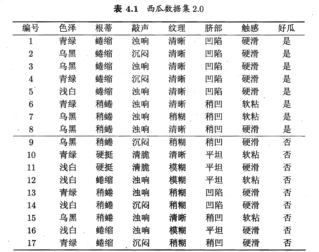
#Calculate the information gain of color attribute
import numpy as np

#The root node information entropy is calculated according to the proportion of good and bad melons
Good = 8
Bad = 9
Total = 17
EntD = - 8/17 * np.log2(8/17) - 9/17 * np.log2(9/17)

#Calculate color information
#Calculate the number of good and bad melons in all colors
Green_good = 3
Green_bad = 3
Black_good = 4
Black_bad = 2
White_good = 1 
White_bad = 4

#Calculate the occurrence probability of good and bad melons
P_Green_good = 3/6
P_Green_bad = 3/6
P_Green = 6/17

P_Black_good = 4/6
P_Black_bad = 2/6
P_Black = 6/17

P_White_good = 1 /5
P_White_bad = 4/5
P_White = 5/17

#Calculate the information entropy of each branch node
EntD_Green = -P_Green_good*np.log2(P_Green_good) -P_Green_bad*np.log2(P_Green_bad)
EntD_White = -P_White_good*np.log2(P_White_good) -P_White_bad*np.log2(P_White_bad)
EntD_Black = -P_Black_good*np.log2(P_Black_good) -P_Black_bad*np.log2(P_Black_bad)

#The information entropy of color attribute is obtained by weighting
EntD_color = P_Green*EntD_Green + P_White*EntD_White + P_Black*EntD_Black

#The information gain of color attribute is obtained by subtraction
Gain = EntD - EntD_color
Gain

0.10812516526536531

According to the above similar method, the information gain of different attributes is calculated.

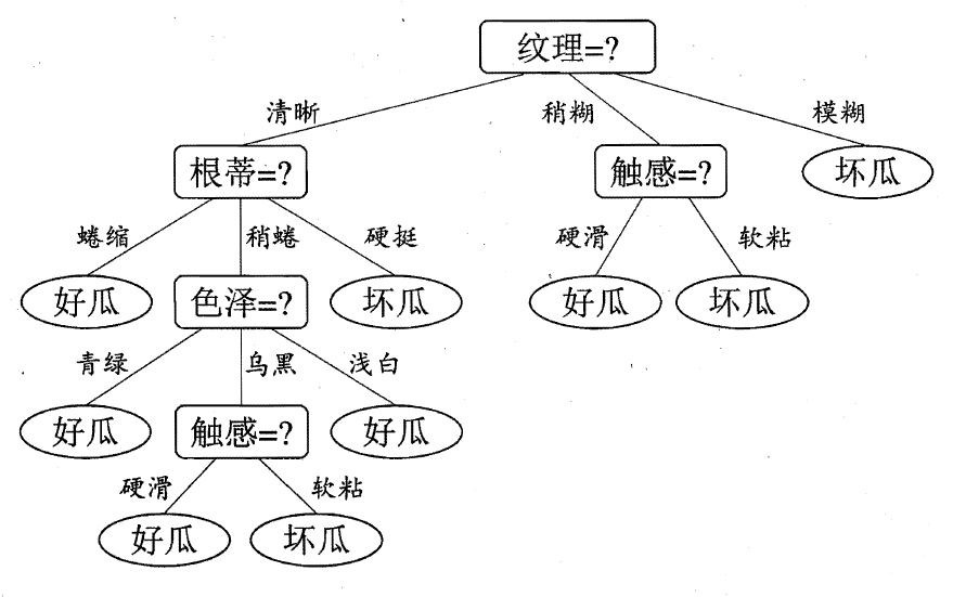
The root node is divided according to the attribute with the largest information gain - texture

Based on the known texture category, the information gain of each attribute is calculated to obtain the decision tree.

2.2 gain rate

The information gain criterion has a preference for attributes with a large number of values.

To solve this problem, Quinlan(1993) used the gain ratio to select the optimal partition attribute, which is defined as follows:

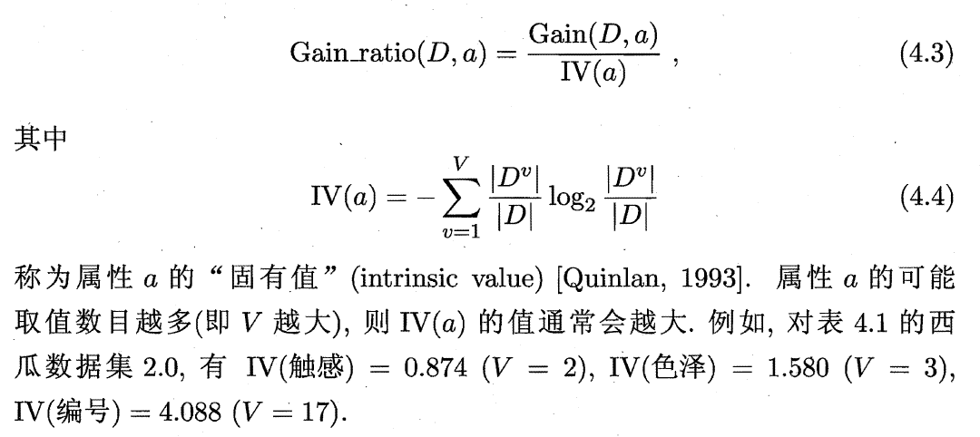
Firstly, the attributes with higher information gain than the average level are found from the candidate partition attributes, and then the number of attribute partition decisions with the highest gain rate is selected.

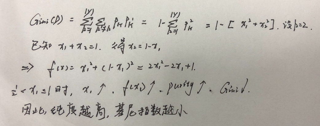
2.3 Gini index

2.3.1 classification tree: Gini index minimum criterion.

Data set Gini index:

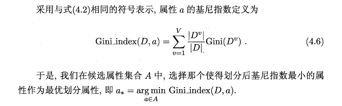
Attribute Gini index:

example

#Gini index of data set: two bifurcation as an example

def gini_index_single(a,b):
    single_gini = 1 - ((a/(a+b))**2) - ((b/(a+b))**2)
    return single_gini

print(gini_index_single(105,39),gini_index_single(130,14))

#It can be seen that the higher the purity, the smaller the Gini index

0.3949652777777779 0.17554012345679013

#Attribute Gini index: weighting of data sets

def gini_index(a, b, c, d):
    zuo = gini_index_single(a,b)
    you = gini_index_single(c,d)
    gini_index = zuo*((a+b)/(a+b+c+d)) + you*((c+d)/(a+b+c+d))
    return gini_index

gini_index(105, 39, 34, 125)

0.36413900824044665

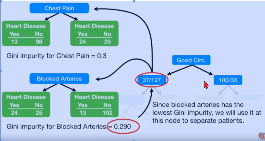
gini_index(37, 127, 100, 33)

0.3600300949466547

gini_index(92, 31, 45, 129)

0.38080175646758213

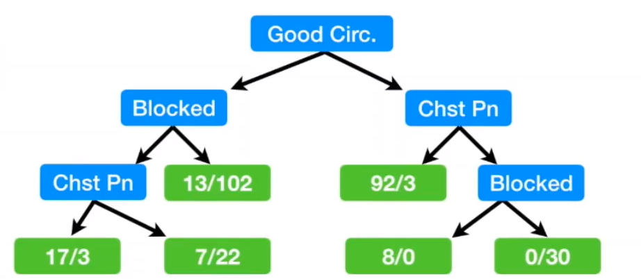
Select the attribute with the smallest Gini index for the first bifurcation, that is, good blood circulation

Continue with the second bifurcation

gini_index_single(37,127)

0.3494199881023201

gini_index(13, 98, 24, 29)

0.30011649938019014

gini_index(24, 25, 13, 102)

0.2899430822169802

According to the above figure, Gini impurity of Blocked arteries is 0.29, which is better than chestpain. (the smaller the Gini index, the better)

And the Gini index after bifurcation is lower than 0.34, so the second bifurcation should be carried out

Therefore, take Blocked arteries as the second bifurcation attribute. Get:

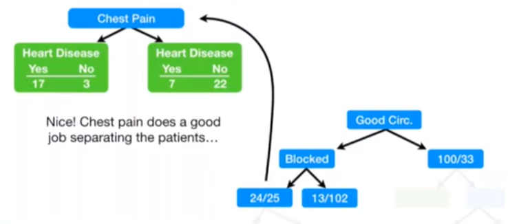
gini_index_single(24, 25)

0.4997917534360683

gini_index(17,3,7,22)

0.3208304011259677

Since 0.32 < 0.49, the third bifurcation should be carried out.

The final bifurcation results are as follows: