Reference City Community
In the task of image segmentation, especially in medical image segmentation, U-Net[1] is undoubtedly one of the most successful methods. This method was proposed at the 2015 MICCAI conference and has been cited more than 4000 times. The structure of encoder (down sampling) - decoder (up sampling) and jump connection is a very classical design method. At present, there are many new convolutional neural network design methods, but many still continue the core idea of U-Net, adding new modules or other design concepts. This paper introduces U-Net and its several improved versions.
U-Net and 3D U-Net
U-Net was originally a convolutional neural network for two-dimensional image segmentation, winning the ISBI 2015 cell tracking challenge and caries detection challenge [2]. A Karas implementation code of U-Net:
https://github.com/zhixuhao/unet
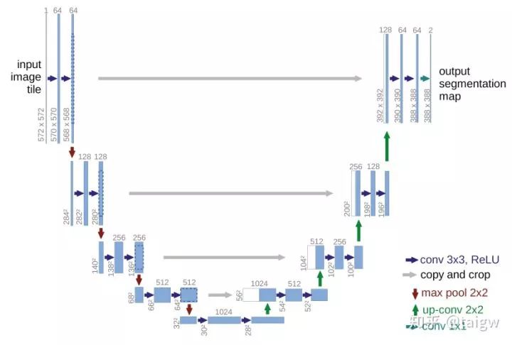
The structure of U-Net is shown in the figure below. The left side can be regarded as an encoder and the right side can be regarded as a decoder. The encoder has four sub modules, each sub module contains two convolution layers, and each sub module is followed by a sub sampling layer implemented by max pool. The resolution of the input image is 572x572, and the resolution of the first and fifth modules are 572x572, 284x284, 140x140, 68x68 and 32x32, respectively. Since the convolution uses the valid mode, the resolution of the latter sub module here is equal to (the resolution of the former sub module - 4) / 2. The decoder consists of four sub modules, and the resolution rises successively through the up sampling operation until it is consistent with the resolution of the input image (because the convolution uses the valid mode, the actual output is smaller than the input image). The network also uses jump connection to connect the up sampling result with the output of the sub module with the same resolution in the encoder as the input of the next sub module in the decoder.
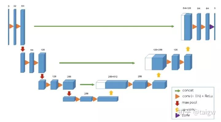
3D U-Net[3] is a simple extension of U-Net, which is applied to 3D image segmentation. The structure is shown in the figure below. Compared with U-Net, the network only uses three subsampling operations, and uses batch normalization after each convolution layer, but neither 3D U-Net nor U-Net uses dropout.
In the 2018 mice brain tumor segmentation challenge (brats) [4], the team of German Cancer Research Center used 3D U-Net, only made a few changes, and achieved the second place in the challenge. It was found that 3D U-Net still has advantages over many new networks [5]. A python implementation of 3D U-Net:
https://github.com/wolny/pytorch-3dunet
TernausNet
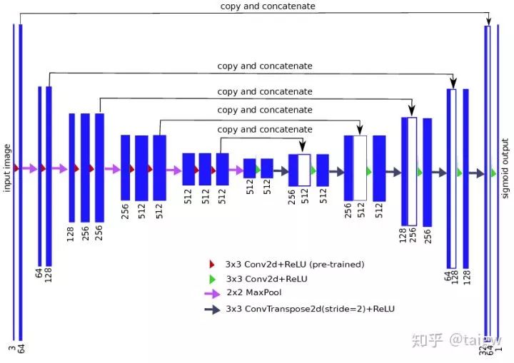
The full name of TernausNet is "TernausNet: U-Net with VGG11 encoder pre trained on ImageNet for image segmentation" [6]. The network replaces the encoder in U-Net with VGG11, and conducts pre training on ImageNet. It stands out from 735 teams and wins the first place in the Carvana Image Masking Challenge. Code link:
https://github.com/ternaus/TernausNet
The following is a schematic diagram of the network:
Res UNET and Dense U-Net
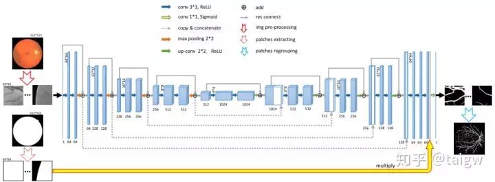
Res UNet and dense UNet are respectively inspired by residual connection and dense connection. Each sub module of UNet is replaced by the form with residual connection and dense connection. [6] Res UNet is used for retinal image segmentation. Its structure is shown in the following figure, where the gray solid line represents the residual connection added in each module.
Dense connection means that the output of a certain layer in the sub module is taken as part of the input of subsequent layers, and the input of a certain layer comes from the combination of the output of previous layers. The figure below is an example of dense connections in [7]. In this paper, the sub modules of U-Net are replaced by such dense connection modules, and full dense UNET is proposed to remove the artifacts in the image.
MultiResUNet
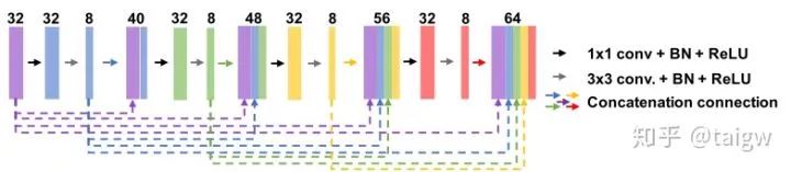
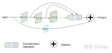
MultiResUNet[8] proposed a MutiRes module combined with UNet. MutiRes module is an extension of residual connection as shown in the figure below. In this module, three convolution results of 3 x 3 are spliced together as a combined feature map, and then added with the result of 1 x 1 convolution of the input feature map.
The structure of the network is shown in the figure below, and the interior of each MultiRes module is shown in the figure above.
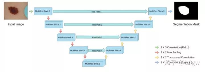
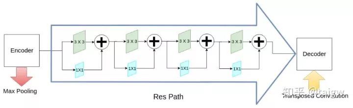
In addition to the MultiRes module, the network also proposes a residual path (ResPath), so that before the encoder features are spliced with the corresponding features in the decoder, some additional convolution operations are carried out, as shown in the figure below. The author thinks that the features in the encoder are low-level features due to the shallow convolution layer, while the corresponding features in the decoder are high-level features due to the deeper convolution layer. There is a big gap between the two in semantics, so it is not suitable to directly splice them. Therefore, an additional ResPath is used to make them have the same depth before splicing. In ResPath1, 2, 3 and 4, 4, 3, 2 and 1 convolutions are used respectively.
In this paper, the performance of ISIC, CVC clinicdb, Brats and other data sets is verified. Code link is
https://github.com/nibtehaz/MultiResUNet
Model code keras; https://github.com/nibtehaz/MultiResUNet/blob/master/MultiResUNet.py
from keras.layers import Input, Conv2D, MaxPooling2D, Conv2DTranspose, concatenate, BatchNormalization, Activation, add
from keras.models import Model, model_from_json
from keras.optimizers import Adam
from keras.layers.advanced_activations import ELU, LeakyReLU
from keras.utils.vis_utils import plot_model


def conv2d_bn(x, filters, num_row, num_col, padding='same', strides=(1, 1), activation='relu', name=None):
    '''
    2D Convolutional layers

    Arguments:
        x {keras layer} -- input layer
        filters {int} -- number of filters
        num_row {int} -- number of rows in filters
        num_col {int} -- number of columns in filters

    Keyword Arguments:
        padding {str} -- mode of padding (default: {'same'})
        strides {tuple} -- stride of convolution operation (default: {(1, 1)})
        activation {str} -- activation function (default: {'relu'})
        name {str} -- name of the layer (default: {None})

    Returns:
        [keras layer] -- [output layer]
    '''

    x = Conv2D(filters, (num_row, num_col), strides=strides, padding=padding, use_bias=False)(x)
    x = BatchNormalization(axis=3, scale=False)(x)

    if(activation == None):
        return x

    x = Activation(activation, name=name)(x)

    return x


def trans_conv2d_bn(x, filters, num_row, num_col, padding='same', strides=(2, 2), name=None):
    '''
    2D Transposed Convolutional layers

    Arguments:
        x {keras layer} -- input layer
        filters {int} -- number of filters
        num_row {int} -- number of rows in filters
        num_col {int} -- number of columns in filters

    Keyword Arguments:
        padding {str} -- mode of padding (default: {'same'})
        strides {tuple} -- stride of convolution operation (default: {(2, 2)})
        name {str} -- name of the layer (default: {None})

    Returns:
        [keras layer] -- [output layer]
    '''

    x = Conv2DTranspose(filters, (num_row, num_col), strides=strides, padding=padding)(x)
    x = BatchNormalization(axis=3, scale=False)(x)

    return x


def MultiResBlock(U, inp, alpha = 1.67):
    '''
    MultiRes Block

    Arguments:
        U {int} -- Number of filters in a corrsponding UNet stage
        inp {keras layer} -- input layer

    Returns:
        [keras layer] -- [output layer]
    '''

    W = alpha * U

    shortcut = inp

    shortcut = conv2d_bn(shortcut, int(W*0.167) + int(W*0.333) +
                         int(W*0.5), 1, 1, activation=None, padding='same')

    conv3x3 = conv2d_bn(inp, int(W*0.167), 3, 3,
                        activation='relu', padding='same')

    conv5x5 = conv2d_bn(conv3x3, int(W*0.333), 3, 3,
                        activation='relu', padding='same')

    conv7x7 = conv2d_bn(conv5x5, int(W*0.5), 3, 3,
                        activation='relu', padding='same')

    out = concatenate([conv3x3, conv5x5, conv7x7], axis=3)
    out = BatchNormalization(axis=3)(out)

    out = add([shortcut, out])
    out = Activation('relu')(out)
    out = BatchNormalization(axis=3)(out)

    return out


def ResPath(filters, length, inp):
    '''
    ResPath

    Arguments:
        filters {int} -- [description]
        length {int} -- length of ResPath
        inp {keras layer} -- input layer

    Returns:
        [keras layer] -- [output layer]
    '''


    shortcut = inp
    shortcut = conv2d_bn(shortcut, filters, 1, 1,
                         activation=None, padding='same')

    out = conv2d_bn(inp, filters, 3, 3, activation='relu', padding='same')

    out = add([shortcut, out])
    out = Activation('relu')(out)
    out = BatchNormalization(axis=3)(out)

    for i in range(length-1):

        shortcut = out
        shortcut = conv2d_bn(shortcut, filters, 1, 1,
                             activation=None, padding='same')

        out = conv2d_bn(out, filters, 3, 3, activation='relu', padding='same')

        out = add([shortcut, out])
        out = Activation('relu')(out)
        out = BatchNormalization(axis=3)(out)

    return out


def MultiResUnet(height, width, n_channels):
    '''
    MultiResUNet

    Arguments:
        height {int} -- height of image
        width {int} -- width of image
        n_channels {int} -- number of channels in image

    Returns:
        [keras model] -- MultiResUNet model
    '''


    inputs = Input((height, width, n_channels))

    mresblock1 = MultiResBlock(32, inputs)
    pool1 = MaxPooling2D(pool_size=(2, 2))(mresblock1)
    mresblock1 = ResPath(32, 4, mresblock1)

    mresblock2 = MultiResBlock(32*2, pool1)
    pool2 = MaxPooling2D(pool_size=(2, 2))(mresblock2)
    mresblock2 = ResPath(32*2, 3, mresblock2)

    mresblock3 = MultiResBlock(32*4, pool2)
    pool3 = MaxPooling2D(pool_size=(2, 2))(mresblock3)
    mresblock3 = ResPath(32*4, 2, mresblock3)

    mresblock4 = MultiResBlock(32*8, pool3)
    pool4 = MaxPooling2D(pool_size=(2, 2))(mresblock4)
    mresblock4 = ResPath(32*8, 1, mresblock4)

    mresblock5 = MultiResBlock(32*16, pool4)

    up6 = concatenate([Conv2DTranspose(
        32*8, (2, 2), strides=(2, 2), padding='same')(mresblock5), mresblock4], axis=3)
    mresblock6 = MultiResBlock(32*8, up6)

    up7 = concatenate([Conv2DTranspose(
        32*4, (2, 2), strides=(2, 2), padding='same')(mresblock6), mresblock3], axis=3)
    mresblock7 = MultiResBlock(32*4, up7)

    up8 = concatenate([Conv2DTranspose(
        32*2, (2, 2), strides=(2, 2), padding='same')(mresblock7), mresblock2], axis=3)
    mresblock8 = MultiResBlock(32*2, up8)

    up9 = concatenate([Conv2DTranspose(32, (2, 2), strides=(
        2, 2), padding='same')(mresblock8), mresblock1], axis=3)
    mresblock9 = MultiResBlock(32, up9)

    conv10 = conv2d_bn(mresblock9, 1, 1, 1, activation='sigmoid')

    model = Model(inputs=[inputs], outputs=[conv10])

    return model
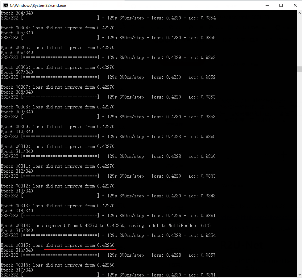
(I have tested this network. With dice loss, the loss has been declining, and the network performance remains doubtful. As shown in the figure below)
R2U-Net
The full name of r2u net is called recurrent recurrent CNN based U-Net [9]. This method combines residual connection and cyclic convolution to replace the original sub module in U-Net, as shown in the figure below
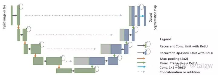
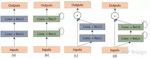
Where a circular arrow indicates a circular connection. The following figure shows the internal structure of several different submodules, (a) is the method used in the conventional U-Net, (b) is the convolution layer containing the activation function on the basis of (a), (c) is the way of using residual connection, (d) is the convolution module combining (b) and (c) proposed in this paper.
The performance of the method is also verified in several public data sets, such as skin disease image, retina image, lung image, etc
https://github.com/LeeJunHyun/Image\_Segmentation#r2u-net
Attention UNet
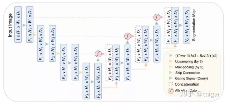
Attention UNet[10] introduces attention mechanism in UNet. Before splicing the features of each resolution of the encoder and the corresponding features of the decoder, an attention module is used to readjust the output features of the encoder. The module generates a gating signal to control the importance of features at different spatial locations, as shown in the red circle in the figure below.
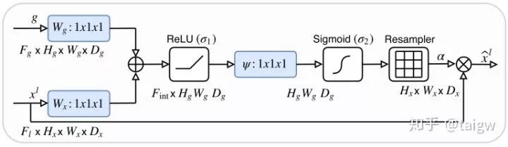
The attention module of the method is shown in the figure below. The module combines the convolution of 1x1x1 with ReLU and Sigmoid respectively to generate a weight graph , which is corrected by multiplying the features in the encoder.
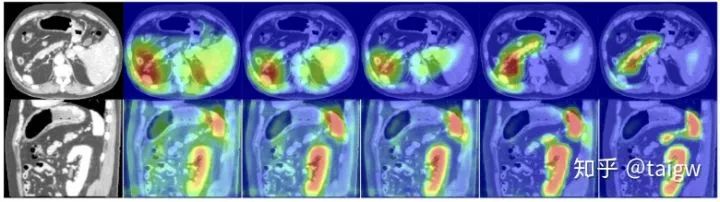
The following figure shows the visualization of the attention weight graph. From left to right are the attention weights of an image and the image as the number of training increases. It can be seen that the obtained attention weight tends to get a large value in the target organ area and a small value in the background area, which is helpful to improve the accuracy of image segmentation.
Code link for this article:
https://github.com/ozan-oktay/Attention-Gated-Networks
other
There are many image segmentation networks designed based on the U-Net framework, which are difficult to list one by one. Here are two more reference articles:
AnatomyNet: Deep 3D Squeeze-and-excitation U-Nets for fast and fully automated whole-volume anatomical segmentation
H-DenseUNet: Hybrid Densely Connected UNet for Liver and Liver Tumor Segmentation from CT Volumes
Refer to ziliao:
http://antkillerfarm.github.io/dl/2018/10/26/Deep_Learning_48.html