Recently, the author studied the Tencent advertising algorithm competition and found that some choices would use GBDT for "dimension reduction" and feature engineering. There are points to be raised, so I'll take a look. A previous article related to LightGBM: python - machine learning lightgbm related practices
Here you can directly run through the github: wangru8080/gbdt-lr
1 GBDT + LR principle
reference resources: GBDT+LR algorithm analysis and Python implementation
1.1 common CTR processes
The most widely used scenario of GBDT+LR is CTR click through rate estimation, that is, to predict whether the advertisements pushed to users will be clicked by users.
The training samples involved in the click through rate prediction model are generally hundreds of millions of levels, with a large sample size. The model often adopts LR with fast speed. However, LR is a linear model with limited learning ability. At this time, feature engineering is particularly important. The existing feature engineering experiments mainly focus on finding distinguishing features and feature combinations. Tossing around may not bring improvement. The characteristics of GBDT algorithm can be used to explore differentiated features and feature combinations, so as to reduce the labor cost in feature engineering.
From know https://zhuanlan.zhihu.com/p/29053940 See a CTR process on the, as shown in the figure below:
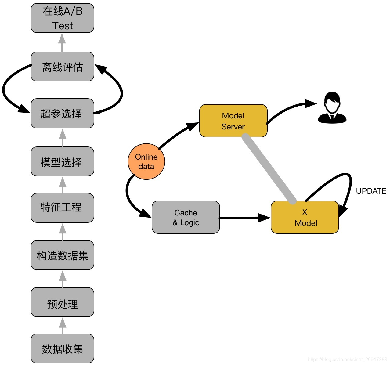
As shown in the figure above, it mainly includes two parts: offline part and online part. The objective of offline part is to train available models, while the online part considers that the performance of the model may decline with time after it is online. In this case, online learning can be used to update the model online
1.2 which is more suitable for RF / gbdt
RF is also a number of trees, but the effect has been proved to be inferior to GBDT. The feature splitting of the tree in front of GBDT mainly reflects the distinguishing feature of most samples; The later trees mainly reflect a few samples with large residual after passing through the first N trees. It is more reasonable to give priority to the features with discrimination on the whole, and then select the features with discrimination for a few samples, which should also be the reason for using GBDT.
1.3 where is gbdt + LR better than FM?
(reading the paper) ctr prediction LR and GBDT+LR model analysis of recommendation system
Although the FM and FFM proposed by feature crossover can better solve the problem of data sparsity, they still stay in the case of second-order crossover.
Facebook proposes a model structure that uses GBDT (Gradient Boosting Decision Tree) to automatically filter and combine features, then generates a new discrete feature vector, and then takes the feature vector as LR model input to predict CTR.
Due to the structural characteristics of decision tree, in fact, the depth of decision tree determines the dimension of feature intersection. If the depth of the decision tree is 4, through three node splitting, the final leaf node is actually the result of third-order feature combination. Obviously, such a strong feature combination ability is not possessed by the model of FM system. However, because GBDT is prone to over fitting and GBDT actually loses a lot of numerical information of features, we can not simply say that GBDT has better effect than FM or FFM due to its stronger ability of feature intersection (in fact, FFM was proposed in 2015). The selection and debugging of the model is always the result of the comprehensive action of many factors.
The significance of GBDT+LR over FM is that it greatly promotes the important trend of feature engineering modeling. In a sense, various network structures for in-depth learning and the application of embedding technology are the continuation of this trend.
1.3 the tree model is poor in processing sparse discrete features
reference resources:
- Tencent big data: GBDT and LR integration scheme in CTR estimation
- Recommendation system meets deep learning (10) – GBDT+LR fusion scheme practice
GBDT is just a memory of history. It has no generalization or generalization ability.
However, this does not mean that for large-scale discrete features, the schemes of GBDT and LR are no longer applicable. If you are interested, you can look at references 2 and 3, which will not be introduced here.
2. Lightgbm + LR integration case
A piece of core code. The overall process is as follows:
Source data - > standardization - > Training LGM model - > predict which node of each tree each sample of training set + verification set falls on ->The node features of LGB are merged into a new training set / verification set
def gbdt_ffm_predict(data, category_feature, continuous_feature):
    # Discrete feature one hot coding
    print('start one-hot...')
    for col in category_feature:
        onehot_feats = pd.get_dummies(data[col], prefix = col)
        data = pd.concat([data, onehot_feats], axis = 1)
    print('one-hot end')


    feats = [col for col in data if col not in category_feature] # onehot_feats + continuous_feature
    tmp = data[feats]
    train = tmp[tmp['Label'] != -1]
    target = train.pop('Label')
    test = tmp[tmp['Label'] == -1]
    test.drop(['Label'], axis = 1, inplace = True)

    # Partition dataset
    print('Partition dataset...')
    x_train, x_val, y_train, y_val = train_test_split(train, target, test_size = 0.2, random_state = 2018)

    print('Start training gbdt..')
    gbm = lgb.LGBMRegressor(objective='binary',
                            subsample= 0.8,
                            min_child_weight= 0.5,
                            colsample_bytree= 0.7,
                            num_leaves=100,
                            max_depth = 12,
                            learning_rate=0.05,
                            n_estimators=10,
                            )

    gbm.fit(x_train, y_train,
            eval_set = [(x_train, y_train), (x_val, y_val)],
            eval_names = ['train', 'val'],
            eval_metric = 'binary_logloss',
            # early_stopping_rounds = 100,
            )
    model = gbm.booster_
    print('Number of leaves obtained by training')
    gbdt_feats_train = model.predict(train, pred_leaf = True)  # Obtain the number of nodes of each tree in the training set (10 trees, 100 leaf nodes per tree)
    train.shape,gbdt_feats_train.shape  # ((1599, 13104), (1599, 10)) dimension reduction from 13104 to 10

    gbdt_feats_test = model.predict(test, pred_leaf = True)    # Obtain the number of nodes of each tree in the validation set (10 trees, 100 leaf nodes per tree)
    gbdt_feats_name = ['gbdt_leaf_' + str(i) for i in range(gbdt_feats_train.shape[1])]
    df_train_gbdt_feats = pd.DataFrame(gbdt_feats_train, columns = gbdt_feats_name)
    df_test_gbdt_feats = pd.DataFrame(gbdt_feats_test, columns = gbdt_feats_name)

    print('Construct a new dataset...')
    tmp = data[category_feature + continuous_feature + ['Label']]
    train = tmp[tmp['Label'] != -1]
    test = tmp[tmp['Label'] == -1]
    train = pd.concat([train, df_train_gbdt_feats], axis = 1)
    test = pd.concat([test, df_test_gbdt_feats], axis = 1)
    data = pd.concat([train, test])
    del train
    del test
    gc.collect()

    # Continuous feature normalization
    print('Start normalization...')
    scaler = MinMaxScaler()
    for col in continuous_feature:
        data[col] = scaler.fit_transform(data[col].values.reshape(-1, 1))
    print('Normalization end')

    data.to_csv('data/data.csv', index = False)
    return category_feature + gbdt_feats_name
Let's take a look at lgbm classifier. For reference: lightgbm.LGBMClassifier As follows:
classlightgbm.LGBMClassifier(boosting_type='gbdt', num_leaves=31, max_depth=- 1, learning_rate=0.1, n_estimators=100, subsample_for_bin=200000, objective=None, class_weight=None, min_split_gain=0.0, min_child_weight=0.001, min_child_samples=20, subsample=1.0, subsample_freq=0, colsample_bytree=1.0, reg_alpha=0.0, reg_lambda=0.0, random_state=None, n_jobs=- 1, silent=True, importance_type='split', **kwargs)
Of which:
- n_estimators - the tree of the tree, equivalent to the principal component, how many principal components are the same
- num_leaves, leaf node
- max_depth (int, optional (default=-1)) – Maximum tree depth for base learners
model.predict(train, pred_leaf = True)_ Leaf (pred_leaf (bool, optional (default = false)) – what to predict leaf index.) can predict the position of each sample at the leaf node:
train.shape,gbdt_feats_train.shape
# ((1599, 13104), (1599, 10))

gbdt_feats_train
>>> array([[ 2,  9,  3, ...,  2, 14,  4],
		       [ 1,  8,  1, ..., 20, 16,  1],
		       [18, 35, 39, ..., 38, 24, 29],
		       ...,
		       [44, 18, 13, ...,  8, 17, 23],
		       [23, 20, 17, ...,  4,  0, 30],
		       [20, 24,  0, ..., 28, 22, 36]])
The dimension is reduced from 13104 to 10 dimensions (trees of the tree), and then each sample is marked at the leaf position of 10 trees (the number of each sample (1599) at the leaf (100 leaves) node of 10 trees)