1.3.4. Target file system
1.3.4.1. Firmware
OpenCL firmware includes pre encapsulated DSP TIDL Library (with hard coded core) and EVE TIDL library following custom accelerator model. OpenCL firmware is downloaded to DSP and M4/EVE immediately after Linux boot:
- dra7-ipu1-fw.xem4 -> /lib/firmware/dra7-ipu1-fw.xem4.opencl-monitor
- dra7-dsp1-fw.xe66 -> /lib/firmware/dra7-dsp1-fw.xe66.opencl-monitor
- dra7-dsp2-fw.xe66 -> /lib/firmware/dra7-dsp2-fw.xe66.opencl-monitor
1.3.4.2. User space components
User space TIDL components are contained in the folder / usr/share/ti/tidl and its subfolders. The subfolder name and description are as follows:
Sub folder	Description of content
examples	    test(File to file example),imagenet Classification, image segmentation and SSD Multiple box examples are here. One based on imagenet Matrix of GUI Example, in tidl_classification Folder.
utils	          For importing models and simulations ARM 32 Bit binaries and configuration files for running the sample import tool operation.
viewer   	Import model parser and point graph creator. Enter yes TIDL Model, output is.dot File, you can use the point tool(x86)convert to PNG or PDF Format.
tidl_api	       TIDL API Source of implementation.
1.3.5. Input data format
The current version is mainly used for 2D input. The most common two-dimensional input tensor is color image. The format must be the same as that used in model training. In general, this follows the BGR plane interleaving format (common in OpenCV). That is, the first two-dimensional array is the blue plane, the second is the green plane, and the last is the red plane.
However, it is entirely possible to input only two planes: for example, one plane with lidar range measurement and the second plane with illumination. This assumes that the same format is used during training.
1.3.6. Output data format
• image classification
There are 1D vectors at the output, one byte for each class (log (softmax)). If the model has 100 classes, the output buffer will be 100 bytes long. If the model has 1000 classes, the output buffer will be 1000 bytes long
• image segmentation
The output buffer is a 2D buffer, usually WxH (width and height of the input image). Each byte is the class index of the pixels in the input image. Typically, the class count is one or two TENS (but must be less than 255)
• target detection
The output buffer is a tuple list, including class index, bounding box (4 parameters) and optional probability measure
1.3.7. Import process
The import process is completed in two steps
• the first step is to parse the model parameters and network topology and convert them into a custom format that TIDL Lib can understand.
• the second step is to calibrate the dynamic quantization process by finding out the activation range of each layer. This is achieved by calling simulation (implemented in native C), which estimates the initial values that are important to the quantization process. Assuming a strong temporal correlation between input frames, these values are then updated by frame.
During the import process, some layers are merged into one TIDL layer (such as volume layer and ReLU layer). This is done to further leverage the EVE architecture, which allows certain operations to be performed free of charge. You can use the TIDL network viewer to check the structure of the transformed (but equivalent) network.
We provide a tool (Linux x86 or ARM Linux port) to import models and parameters trained on PC using caffe framework or tensor flow framework. The tool accepts various parameters through importing configuration files and generates model and parameter files. The code will be executed across multiple EVE and DSP cores using TIDL library. The import configuration file is located in {TIDL_install_path} / test / testecs / config / import
1.3.7.3. Import tool tracking
During the conversion process, the import tool generates tracks and reports the detected layers and their parameters (the last columns represent the input tensor dimension and the output tensor dimension).
Processing config file ./tempDir/qunat_stats_config.txt !
0, TIDL_DataLayer                 ,  0,  -1 ,  1 ,  x ,  x ,  x ,  x ,  x ,  x ,  x ,  x ,  0 ,    0 ,    0 ,    0 ,    0 ,    1 ,    3 ,  224 ,  224 ,
1, TIDL_BatchNormLayer            ,  1,   1 ,  1 ,  0 ,  x ,  x ,  x ,  x ,  x ,  x ,  x ,  1 ,    1 ,    3 ,  224 ,  224 ,    1 ,    3 ,  224 ,  224 ,
2, TIDL_ConvolutionLayer          ,  1,   1 ,  1 ,  1 ,  x ,  x ,  x ,  x ,  x ,  x ,  x ,  2 ,    1 ,    3 ,  224 ,  224 ,    1 ,   32 ,  112 ,  112 ,
3, TIDL_ConvolutionLayer          ,  1,   1 ,  1 ,  2 ,  x ,  x ,  x ,  x ,  x ,  x ,  x ,  3 ,    1 ,   32 ,  112 ,  112 ,    1 ,   32 ,   56 ,   56 ,
4, TIDL_ConvolutionLayer          ,  1,   1 ,  1 ,  3 ,  x ,  x ,  x ,  x ,  x ,  x ,  x ,  4 ,    1 ,   32 ,   56 ,   56 ,    1 ,   64 ,   56 ,   56 ,
5, TIDL_ConvolutionLayer          ,  1,   1 ,  1 ,  4 ,  x ,  x ,  x ,  x ,  x ,  x ,  x ,  5 ,    1 ,   64 ,   56 ,   56 ,    1 ,   64 ,   28 ,   28 ,
6, TIDL_ConvolutionLayer          ,  1,   1 ,  1 ,  5 ,  x ,  x ,  x ,  x ,  x ,  x ,  x ,  6 ,    1 ,   64 ,   28 ,   28 ,    1 ,  128 ,   28 ,   28 ,
7, TIDL_ConvolutionLayer          ,  1,   1 ,  1 ,  6 ,  x ,  x ,  x ,  x ,  x ,  x ,  x ,  7 ,    1 ,  128 ,   28 ,   28 ,    1 ,  128 ,   14 ,   14 ,
8, TIDL_ConvolutionLayer          ,  1,   1 ,  1 ,  7 ,  x ,  x ,  x ,  x ,  x ,  x ,  x ,  8 ,    1 ,  128 ,   14 ,   14 ,    1 ,  256 ,   14 ,   14 ,
9, TIDL_ConvolutionLayer          ,  1,   1 ,  1 ,  8 ,  x ,  x ,  x ,  x ,  x ,  x ,  x ,  9 ,    1 ,  256 ,   14 ,   14 ,    1 ,  256 ,    7 ,    7 ,
10, TIDL_ConvolutionLayer         ,  1,   1 ,  1 ,  9 ,  x ,  x ,  x ,  x ,  x ,  x ,  x , 10 ,    1 ,  256 ,    7 ,    7 ,    1 ,  512 ,    7 ,    7 ,
11, TIDL_ConvolutionLayer         ,  1,   1 ,  1 , 10 ,  x ,  x ,  x ,  x ,  x ,  x ,  x , 11 ,    1 ,  512 ,    7 ,    7 ,    1 ,  512 ,    7 ,    7 ,
12, TIDL_PoolingLayer             ,  1,   1 ,  1 , 11 ,  x ,  x ,  x ,  x ,  x ,  x ,  x , 12 ,    1 ,  512 ,    7 ,    7 ,    1 ,    1 ,    1 ,  512 ,
13, TIDL_InnerProductLayer        ,  1,   1 ,  1 , 12 ,  x ,  x ,  x ,  x ,  x ,  x ,  x , 13 ,    1 ,    1 ,    1 ,  512 ,    1 ,    1 ,    1 ,    9 ,
14, TIDL_SoftMaxLayer             ,  1,   1 ,  1 , 13 ,  x ,  x ,  x ,  x ,  x ,  x ,  x , 14 ,    1 ,    1 ,    1 ,    9 ,    1 ,    1 ,    1 ,    9 ,
15, TIDL_DataLayer                ,  0,   1 , -1 , 14 ,  x ,  x ,  x ,  x ,  x ,  x ,  x ,  0 ,    1 ,    1 ,    1 ,    9 ,    0 ,    0 ,    0 ,    0 ,
Layer ID    ,inBlkWidth  ,inBlkHeight ,inBlkPitch  ,outBlkWidth ,outBlkHeight,outBlkPitch ,numInChs    ,numOutChs   ,numProcInChs,numLclInChs ,numLclOutChs,numProcItrs ,numAccItrs  ,numHorBlock ,numVerBlock ,inBlkChPitch,outBlkChPitc,alignOrNot
  2           72           64           72           32           28           32            3           32            3            1            8            1            3            4            4         4608          896            1
  3           40           30           40           32           28           32            8            8            8            4            8            1            2            4            4         1200          896            1
  4           40           30           40           32           28           32           32           64           32            7            8            1            5            2            2         1200          896            1
  5           40           30           40           32           28           32           16           16           16            7            8            1            3            2            2         1200          896            1
  6           40           30           40           32           28           32           64          128           64            7            8            1           10            1            1         1200          896            1
  7           40           30           40           32           28           32           32           32           32            7            8            1            5            1            1         1200          896            1
  8           24           16           24           16           14           16          128          256          128            8            8            1           16            1            1          384          224            1
  9           24           16           24           16           14           16           64           64           64            8            8            1            8            1            1          384          224            1
 10           24            9           24           16            7           16          256          512          256            8            8            1           32            1            1          216          112            1
 11           24            9           24           16            7           16          128          128          128            8            8            1           16            1            1          216          112            1
  Processing Frame Number : 0
The final output (based on the calibration original image provided in the configuration file) is stored in a file with a reserved name: stats_tool_out.bin. The size of this file should be the same as the output class count (in the case of classification). For example, for imagenet 1000 class, it must be 1000 bytes. Except for final blob, all intermediate results (activation of a single layer) Are stored in the. / tempDir folder (in the folder where import is called). The following is an example list of files with intermediate activation:
•	trace_dump_0_224x224.y <- This very first layer should be identical to the data blob used in desktop Caffe (during validation)
•	trace_dump_1_224x224.y
•	trace_dump_2_112x112.y
•	trace_dump_3_56x56.y
•	trace_dump_4_56x56.y
•	trace_dump_5_28x28.y
•	trace_dump_6_28x28.y
•	trace_dump_7_14x14.y
•	trace_dump_8_14x14.y
•	trace_dump_9_7x7.y
•	trace_dump_10_7x7.y
•	trace_dump_11_7x7.y
•	trace_dump_12_512x1.y
•	trace_dump_13_9x1.y
•	trace_dump_14_9x1.y
1.3.7.4. Split layers between layer groups
In order to use DSP and EVE accelerator at the same time, the concept of layer group can be used to divide the network into two subgraphs. Multiple layer groups can be executed on EVE and another layer group can be executed on DSP. The output of the first group (running on EVE) will be used as the input of DSP.
This can be achieved by (providing an example of Jacinto11 network):
# Default - 0
randParams         = 0

# 0: Caffe, 1: TensorFlow, Default - 0
modelType          = 0

# 0: Fixed quantization By tarininng Framework, 1: Dynamic quantization by TIDL, Default - 1
quantizationStyle  = 1

# quantRoundAdd/100 will be added while rounding to integer, Default - 50
quantRoundAdd      = 25

numParamBits       = 8
# 0 : 8bit Unsigned, 1 : 8bit Signed Default - 1
inElementType      = 0

inputNetFile       = "../caffe_jacinto_models/trained/image_classification/imagenet_jacintonet11v2/sparse/deploy.prototxt"
inputParamsFile    = "../caffe_jacinto_models/trained/image_classification/imagenet_jacintonet11v2/sparse/imagenet_jacintonet11v2_iter_160000.caffemodel"
outputNetFile      = "./tidl_models/tidl_net_imagenet_jacintonet11v2.bin"
outputParamsFile   = "./tidl_models/tidl_param_imagenet_jacintonet11v2.bin"

sampleInData = "./input/preproc_0_224x224.y"
tidlStatsTool = "./bin/eve_test_dl_algo_ref.out"
layersGroupId    = 0       1       1       1       1       1       1       1       1       1       1       1       2       2       2       0
conv2dKernelType = 0       0       0       0       0       0       0       0       0       0       0       0       1       1       1       1
The input and output layers belong to layer group 0. Layer group 1 is assigned to EVE and layer group 2 is assigned to DSP.
The second line (conv2dKernelType) indicates whether the calculation is sparse (0) or dense (1).
After conversion, we can visualize the network:
tidl_viewer -p -d ./j11split.dot ./tidl_net_imagenet_jacintonet11v2.bin
dot -Tpdf ./j11split.dot -o ./j11split.pdf
The following figure (group 1 is executed on EVE and group 2 is executed on DSP):
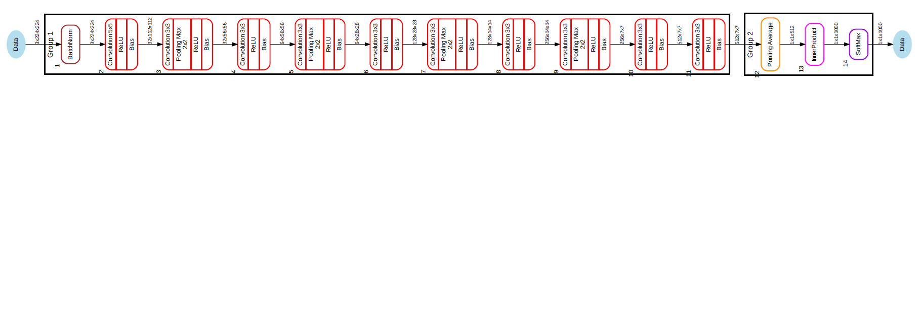
The output of layer group 1 is shared (common) with the input buffer of layer group 2, so there is no additional buffer replication overhead. Due to this buffer allocation, the sequential operation of EVE and DSP is necessary.
1.3.7.5. Theoretical GMAC required for calculation
For the most densely calculated layers (convolution layer and fully connected layer), this can be calculated in advance. Each convolution layer has a certain number of input and output feature maps (2D tensors). The input feature maps are convoluted with convolution kernel (usually 3x3, but also 5x5, 7x7...) Therefore, the total number of MACS can be calculated as: Height_input_map x Width_input_map x N_input_maps x N_output_maps x size_of_kernel.
E.g. for 112x112 feature map, with 64 inputs, 64 outputs and 3x3 kernels, we need:
112x112x64x64x3x3 MAC operations = 4624229916 MAC operations
Similarly, for the full connection layer, the total number of MAC operations of N_inputs and N_outputs is
E.g. N_inputs = 4096 and N_outputs = 1000,
Fully Connected Layer MAC operations = N_inputs * N_outputs = 4096 * 1000 = 4096000 MAC operations
Obviously, the workload of the convolution layer is significantly higher.
1.3.7.6. Mapping to EVE function
Each EVE kernel can perform 16 MAC operations per cycle. The accumulated results are stored in a 40 bit accumulator and can be bucket shifted before being stored in local memory. In addition, EVE can perform ReLU operations for free, so it often combines the volume layer or full connection layer with ReLU.
To support these operations, a wide path to local memory is required. Concurrent transfers from external DDR memory are performed using a dedicated EDMA engine. Therefore, when EVE performs convolution, it always accesses the activation and weight already existing in high-speed local memory at the same time.
One or two layers are implemented on EVE's local RISC CPU and are mainly used for vector engine and EDMA programming. In these rare cases, EVE CPU is used as a fully programmable but slow computing engine. SoftMax layer is implemented using general-purpose CPU and is much slower than DSP or A15. Since SoftMax layer is a terminal layer, it is recommended to use A15 (in user space) or DSP Execute SoftMax on (layergroup2, as implemented in the JDetNet example).
1.3.8. Viewer tool
The viewer tool visualizes the imported network model. For more details, visit https://software-dl.ti.com/mctools/esd/docs/tidl-api/viewer.html The following is an example command line:
root@am57xx-evm:/usr/share/ti/tidl/examples/test/testvecs/config/tidl_models# tidl_viewer
Usage: tidl_viewer -d <dot file name> <network binary file>
Version: 01.00.00.02.7b65cbb
Options:
-p              Print network layer info
-h              Display this help message


root@am57xx-evm:/usr/share/ti/tidl/examples/test/testvecs/config/tidl_models# tidl_viewer -p -d ./jacinto11.dot ./tidl_net_imagenet_jacintonet11v2.bin
  #  Name                  gId   #i   #o   i0   i1   i2   i3   i4   i5   i6   i7   o   #roi    #ch      h      w   #roi    #ch      h      w
  0, Data                ,  0,  -1 ,  1 ,  x ,  x ,  x ,  x ,  x ,  x ,  x ,  x ,  0 ,    0 ,    0 ,    0 ,    0 ,    1 ,    3 ,  224 ,  224 ,
  1, BatchNorm           ,  1,   1 ,  1 ,  0 ,  x ,  x ,  x ,  x ,  x ,  x ,  x ,  1 ,    1 ,    3 ,  224 ,  224 ,    1 ,    3 ,  224 ,  224 ,
  2, Convolution         ,  1,   1 ,  1 ,  1 ,  x ,  x ,  x ,  x ,  x ,  x ,  x ,  2 ,    1 ,    3 ,  224 ,  224 ,    1 ,   32 ,  112 ,  112 ,
  3, Convolution         ,  1,   1 ,  1 ,  2 ,  x ,  x ,  x ,  x ,  x ,  x ,  x ,  3 ,    1 ,   32 ,  112 ,  112 ,    1 ,   32 ,   56 ,   56 ,
  4, Convolution         ,  1,   1 ,  1 ,  3 ,  x ,  x ,  x ,  x ,  x ,  x ,  x ,  4 ,    1 ,   32 ,   56 ,   56 ,    1 ,   64 ,   56 ,   56 ,
  5, Convolution         ,  1,   1 ,  1 ,  4 ,  x ,  x ,  x ,  x ,  x ,  x ,  x ,  5 ,    1 ,   64 ,   56 ,   56 ,    1 ,   64 ,   28 ,   28 ,
  6, Convolution         ,  1,   1 ,  1 ,  5 ,  x ,  x ,  x ,  x ,  x ,  x ,  x ,  6 ,    1 ,   64 ,   28 ,   28 ,    1 ,  128 ,   28 ,   28 ,
  7, Convolution         ,  1,   1 ,  1 ,  6 ,  x ,  x ,  x ,  x ,  x ,  x ,  x ,  7 ,    1 ,  128 ,   28 ,   28 ,    1 ,  128 ,   14 ,   14 ,
  8, Convolution         ,  1,   1 ,  1 ,  7 ,  x ,  x ,  x ,  x ,  x ,  x ,  x ,  8 ,    1 ,  128 ,   14 ,   14 ,    1 ,  256 ,   14 ,   14 ,
  9, Convolution         ,  1,   1 ,  1 ,  8 ,  x ,  x ,  x ,  x ,  x ,  x ,  x ,  9 ,    1 ,  256 ,   14 ,   14 ,    1 ,  256 ,    7 ,    7 ,
  10, Convolution         ,  1,   1 ,  1 ,  9 ,  x ,  x ,  x ,  x ,  x ,  x ,  x , 10 ,    1 ,  256 ,    7 ,    7 ,    1 ,  512 ,    7 ,    7 ,
  11, Convolution         ,  1,   1 ,  1 , 10 ,  x ,  x ,  x ,  x ,  x ,  x ,  x , 11 ,    1 ,  512 ,    7 ,    7 ,    1 ,  512 ,    7 ,    7 ,
  12, Pooling             ,  1,   1 ,  1 , 11 ,  x ,  x ,  x ,  x ,  x ,  x ,  x , 12 ,    1 ,  512 ,    7 ,    7 ,    1 ,    1 ,    1 ,  512 ,
  13, InnerProduct        ,  1,   1 ,  1 , 12 ,  x ,  x ,  x ,  x ,  x ,  x ,  x , 13 ,    1 ,    1 ,    1 ,  512 ,    1 ,    1 ,    1 , 1000 ,
  14, SoftMax             ,  1,   1 ,  1 , 13 ,  x ,  x ,  x ,  x ,  x ,  x ,  x , 14 ,    1 ,    1 ,    1 , 1000 ,    1 ,    1 ,    1 , 1000 ,
  15, Data                ,  0,   1 , -1 , 14 ,  x ,  x ,  x ,  x ,  x ,  x ,  x ,  0 ,    1 ,    1 ,    1 , 1000 ,    0 ,    0 ,    0 ,    0 ,
The output file is jacinto11.dot, which can be converted to PNG or PDF files on Linux x86. Use (for example):
dot -Tpdf ./jacinto11.dot -o ./jacinto11.pdf
• point to the layer group in JDetNet and describe how to divide the graph into two groups to create EVE optimal group and DSP optimal group
1.3.9. Simulation tools
We provide PLSDK ARM file system simulation tool and Linux x86 simulation tool. This is an accurate bit simulation, so the output of the simulation tool should be the same as that of the A5749 or AM57xx target. Use this tool only as a convenience tool (for example, testing a model on a setup without a target EVM).
The simulation tool can also be used to verify the accuracy of the conversion model (FP32 and 8-bit Implementation). It can run in parallel with more kernels on x86 (the simulation tool is a single threaded Implementation). Due to bit accurate simulation, the performance of the simulation tool can not be used to predict the target execution time, but can be used to verify the accuracy of the model.
An example of a configuration file, which includes the specification of processing frame number, input image file (with one or more original images), numerical format of input image file (signed or unsigned), tracking folder and model file:
rawImage    = 1
numFrames   = 1
inData   = "./tmp.raw"
inElementType      = 0
traceDumpBaseName   = "./out/trace_dump_"
outData   = "stats_tool_out.bin"
netBinFile      = "./tidl_net_imagenet_jacintonet11v2.bin"
paramsBinFile   = "./tidl_param_imagenet_jacintonet11v2.bin"
If you need to process multiple images, you can use the following (or similar) script:
 SRC_DIR=$1

 echo "#########################################################" >  TestResults.log
 echo "Testing in $SRC_DIR" >> TestResults.log
 echo "#########################################################" >> TestResults.log
 for filename in $SRC_DIR/*.png; do
  convert $filename -separate +channel -swap 0,2 -combine -colorspace sRGB ./sample_bgr.png
      convert ./sample_bgr.png  -interlace plane BGR:sample_img_256x256.raw
      ./eve_test_dl_algo.out sim.txt
      echo "$filename Results " >> TestResults.log
      hd stats_tool_out.bin | tee -a TestResults.log
done
Simulation tool. / eve_test_dl_algo.out is called with a single command line argument:
./eve_test_dl_algo.out sim.txt
The simulation profile includes a list of network modes to execute, in which case there is only one: tild_config_j11.txt list ends with "0":
1 ./tidl_config_j11_v2.txt
0
Sample configuration file used by simulation tool (tidl_config_j11_v2.txt):
rawImage    = 1
numFrames   = 1
preProcType  = 0
inData   = "./sample_img_256x256.raw"
traceDumpBaseName   = "./out/trace_dump_"
outData   = "stats_tool_out.bin"
updateNetWithStats   = 0
netBinFile      = "./tidl_net_model.bin"
paramsBinFile   = "./tidl_param_model.bin"
SRC_ The results of all images in dir will be directed to TestResults.log and can be tested in caffe Jacinto desktop execution
1.3.10. Overview of model migration steps
• after creating a model using a desktop framework (cafe or TF), it is necessary to verify the accuracy of the model (using reasoning on the desktop framework: Cafe / Cafe Jacinto or TensorFlow).
• import the final model using the above import procedure (for caffe Jacinto, at the end of the "sparse" phase)
• use simulation tools to verify accuracy (using smaller test data sets than those used in the first step) and the decrease in accuracy (relative to the first step) should not be too large (a few percent).
• test the network on the target using TIDL API based programs and imported models.