Three ways of feature dimension reduction

Keywords: Python

Dimension reduction actually reduces the number of features, and the end result is that there is no correlation between the features and the features.

Dimension reduction: Dimension reduction refers to the process of reducing the number of random variables (characteristics) to obtain a set of "unrelated" principal variables under certain restricted conditions.

Two ways to reduce dimensions:

1. Feature Selection

2. Principal Component Analysis (can be understood as a feature extraction method)

1. Feature Selection

Definition: Data contains redundant or related variables (or features, attributes, indicators, etc.) designed to identify key characteristics from existing ones

2 methods for feature selection (filter + embedded)

Filter: mainly explores the characteristics of the feature itself, the relationship between the features and the target values.

    Variance Selection: Low variance feature filtering. For example, it is inappropriate whether a bird can fly as an eigenvalue, where the variance is 0

    Coefficient of correlation: The goal is to remove redundancy and determine the correlation between features and features

Embedded: The algorithm automatically selects features (the association between features and target values)

    Decision Tree: Information Entropy, Information Gain

    Regularization: L1, L2

    In-depth learning: convolution, etc.

Modular

sklearn.feature_selection

1. Dimension Reduction Method 1: Feature Selection - Filtering - Low Variance Filtering

Low variance feature filtering

Delete some features of the low variance and consider how the variance is large.

Small variance of features: most samples of a feature have similar values

Large variance of features: Many samples of a feature have different values

API

sklearn.feature_selection.VarianceThreshold( threshold = 0.0 )

    Delete all low variance features

    Variance.fit_transform(X)

        Data in X:numpy array format [n_samples, n_features]

        Return: Features with training set differences lower than threshold s will be deleted.The default value is to preserve all non-zero variance features, that is, to delete features with the same values in all samples.

#Delete Low Variance Features Demo

from sklearn.datasets import load_iris
from sklearn.feature_selection import VarianceThreshold
import pandas as pd

def variance_demo():
    iris = load_iris()
    data = pd.DataFrame(iris.data, columns = iris.feature_names)
    data_new = data.iloc[:, :4].values
    
    print("data_new:\n", data_new)
    
    transfer = VarianceThreshold(threshold = 0.5)
    
    data_variance_value = transfer.fit_transform(data_new)
    print("data_variance_value:\n", data_variance_value)
    
    return None

if __name__ == '__main__':
    variance_demo()





//Output results:
data_new:
 [[5.1 3.5 1.4 0.2]
 [4.9 3.  1.4 0.2]
 [4.7 3.2 1.3 0.2]
 [4.6 3.1 1.5 0.2]
 [5.  3.6 1.4 0.2]
 [5.4 3.9 1.7 0.4]
 [4.6 3.4 1.4 0.3]
 [5.  3.4 1.5 0.2]
 [4.4 2.9 1.4 0.2]
 [4.9 3.1 1.5 0.1]
 [5.4 3.7 1.5 0.2]
 [4.8 3.4 1.6 0.2]
 [4.8 3.  1.4 0.1]
 [4.3 3.  1.1 0.1]
 [5.8 4.  1.2 0.2]
 [5.7 4.4 1.5 0.4]
 [5.4 3.9 1.3 0.4]
 [5.1 3.5 1.4 0.3]
 [5.7 3.8 1.7 0.3]
 [5.1 3.8 1.5 0.3]
 [5.4 3.4 1.7 0.2]
 [5.1 3.7 1.5 0.4]
 [4.6 3.6 1.  0.2]
 [5.1 3.3 1.7 0.5]
 [4.8 3.4 1.9 0.2]
 [5.  3.  1.6 0.2]
 [5.  3.4 1.6 0.4]
 [5.2 3.5 1.5 0.2]
 [5.2 3.4 1.4 0.2]
 [4.7 3.2 1.6 0.2]
 [4.8 3.1 1.6 0.2]
 [5.4 3.4 1.5 0.4]
 [5.2 4.1 1.5 0.1]
 [5.5 4.2 1.4 0.2]
 [4.9 3.1 1.5 0.1]
 [5.  3.2 1.2 0.2]
 [5.5 3.5 1.3 0.2]
 [4.9 3.1 1.5 0.1]
 [4.4 3.  1.3 0.2]
 [5.1 3.4 1.5 0.2]
 [5.  3.5 1.3 0.3]
 [4.5 2.3 1.3 0.3]
 [4.4 3.2 1.3 0.2]
 [5.  3.5 1.6 0.6]
 [5.1 3.8 1.9 0.4]
 [4.8 3.  1.4 0.3]
 [5.1 3.8 1.6 0.2]
 [4.6 3.2 1.4 0.2]
 [5.3 3.7 1.5 0.2]
 [5.  3.3 1.4 0.2]
 [7.  3.2 4.7 1.4]
 [6.4 3.2 4.5 1.5]
 [6.9 3.1 4.9 1.5]
 [5.5 2.3 4.  1.3]
 [6.5 2.8 4.6 1.5]
 [5.7 2.8 4.5 1.3]
 [6.3 3.3 4.7 1.6]
 [4.9 2.4 3.3 1. ]
 [6.6 2.9 4.6 1.3]
 [5.2 2.7 3.9 1.4]
 [5.  2.  3.5 1. ]
 [5.9 3.  4.2 1.5]
 [6.  2.2 4.  1. ]
 [6.1 2.9 4.7 1.4]
 [5.6 2.9 3.6 1.3]
 [6.7 3.1 4.4 1.4]
 [5.6 3.  4.5 1.5]
 [5.8 2.7 4.1 1. ]
 [6.2 2.2 4.5 1.5]
 [5.6 2.5 3.9 1.1]
 [5.9 3.2 4.8 1.8]
 [6.1 2.8 4.  1.3]
 [6.3 2.5 4.9 1.5]
 [6.1 2.8 4.7 1.2]
 [6.4 2.9 4.3 1.3]
 [6.6 3.  4.4 1.4]
 [6.8 2.8 4.8 1.4]
 [6.7 3.  5.  1.7]
 [6.  2.9 4.5 1.5]
 [5.7 2.6 3.5 1. ]
 [5.5 2.4 3.8 1.1]
 [5.5 2.4 3.7 1. ]
 [5.8 2.7 3.9 1.2]
 [6.  2.7 5.1 1.6]
 [5.4 3.  4.5 1.5]
 [6.  3.4 4.5 1.6]
 [6.7 3.1 4.7 1.5]
 [6.3 2.3 4.4 1.3]
 [5.6 3.  4.1 1.3]
 [5.5 2.5 4.  1.3]
 [5.5 2.6 4.4 1.2]
 [6.1 3.  4.6 1.4]
 [5.8 2.6 4.  1.2]
 [5.  2.3 3.3 1. ]
 [5.6 2.7 4.2 1.3]
 [5.7 3.  4.2 1.2]
 [5.7 2.9 4.2 1.3]
 [6.2 2.9 4.3 1.3]
 [5.1 2.5 3.  1.1]
 [5.7 2.8 4.1 1.3]
 [6.3 3.3 6.  2.5]
 [5.8 2.7 5.1 1.9]
 [7.1 3.  5.9 2.1]
 [6.3 2.9 5.6 1.8]
 [6.5 3.  5.8 2.2]
 [7.6 3.  6.6 2.1]
 [4.9 2.5 4.5 1.7]
 [7.3 2.9 6.3 1.8]
 [6.7 2.5 5.8 1.8]
 [7.2 3.6 6.1 2.5]
 [6.5 3.2 5.1 2. ]
 [6.4 2.7 5.3 1.9]
 [6.8 3.  5.5 2.1]
 [5.7 2.5 5.  2. ]
 [5.8 2.8 5.1 2.4]
 [6.4 3.2 5.3 2.3]
 [6.5 3.  5.5 1.8]
 [7.7 3.8 6.7 2.2]
 [7.7 2.6 6.9 2.3]
 [6.  2.2 5.  1.5]
 [6.9 3.2 5.7 2.3]
 [5.6 2.8 4.9 2. ]
 [7.7 2.8 6.7 2. ]
 [6.3 2.7 4.9 1.8]
 [6.7 3.3 5.7 2.1]
 [7.2 3.2 6.  1.8]
 [6.2 2.8 4.8 1.8]
 [6.1 3.  4.9 1.8]
 [6.4 2.8 5.6 2.1]
 [7.2 3.  5.8 1.6]
 [7.4 2.8 6.1 1.9]
 [7.9 3.8 6.4 2. ]
 [6.4 2.8 5.6 2.2]
 [6.3 2.8 5.1 1.5]
 [6.1 2.6 5.6 1.4]
 [7.7 3.  6.1 2.3]
 [6.3 3.4 5.6 2.4]
 [6.4 3.1 5.5 1.8]
 [6.  3.  4.8 1.8]
 [6.9 3.1 5.4 2.1]
 [6.7 3.1 5.6 2.4]
 [6.9 3.1 5.1 2.3]
 [5.8 2.7 5.1 1.9]
 [6.8 3.2 5.9 2.3]
 [6.7 3.3 5.7 2.5]
 [6.7 3.  5.2 2.3]
 [6.3 2.5 5.  1.9]
 [6.5 3.  5.2 2. ]
 [6.2 3.4 5.4 2.3]
 [5.9 3.  5.1 1.8]]
data_variance_value:
 [[5.1 1.4 0.2]
 [4.9 1.4 0.2]
 [4.7 1.3 0.2]
 [4.6 1.5 0.2]
 [5.  1.4 0.2]
 [5.4 1.7 0.4]
 [4.6 1.4 0.3]
 [5.  1.5 0.2]
 [4.4 1.4 0.2]
 [4.9 1.5 0.1]
 [5.4 1.5 0.2]
 [4.8 1.6 0.2]
 [4.8 1.4 0.1]
 [4.3 1.1 0.1]
 [5.8 1.2 0.2]
 [5.7 1.5 0.4]
 [5.4 1.3 0.4]
 [5.1 1.4 0.3]
 [5.7 1.7 0.3]
 [5.1 1.5 0.3]
 [5.4 1.7 0.2]
 [5.1 1.5 0.4]
 [4.6 1.  0.2]
 [5.1 1.7 0.5]
 [4.8 1.9 0.2]
 [5.  1.6 0.2]
 [5.  1.6 0.4]
 [5.2 1.5 0.2]
 [5.2 1.4 0.2]
 [4.7 1.6 0.2]
 [4.8 1.6 0.2]
 [5.4 1.5 0.4]
 [5.2 1.5 0.1]
 [5.5 1.4 0.2]
 [4.9 1.5 0.1]
 [5.  1.2 0.2]
 [5.5 1.3 0.2]
 [4.9 1.5 0.1]
 [4.4 1.3 0.2]
 [5.1 1.5 0.2]
 [5.  1.3 0.3]
 [4.5 1.3 0.3]
 [4.4 1.3 0.2]
 [5.  1.6 0.6]
 [5.1 1.9 0.4]
 [4.8 1.4 0.3]
 [5.1 1.6 0.2]
 [4.6 1.4 0.2]
 [5.3 1.5 0.2]
 [5.  1.4 0.2]
 [7.  4.7 1.4]
 [6.4 4.5 1.5]
 [6.9 4.9 1.5]
 [5.5 4.  1.3]
 [6.5 4.6 1.5]
 [5.7 4.5 1.3]
 [6.3 4.7 1.6]
 [4.9 3.3 1. ]
 [6.6 4.6 1.3]
 [5.2 3.9 1.4]
 [5.  3.5 1. ]
 [5.9 4.2 1.5]
 [6.  4.  1. ]
 [6.1 4.7 1.4]
 [5.6 3.6 1.3]
 [6.7 4.4 1.4]
 [5.6 4.5 1.5]
 [5.8 4.1 1. ]
 [6.2 4.5 1.5]
 [5.6 3.9 1.1]
 [5.9 4.8 1.8]
 [6.1 4.  1.3]
 [6.3 4.9 1.5]
 [6.1 4.7 1.2]
 [6.4 4.3 1.3]
 [6.6 4.4 1.4]
 [6.8 4.8 1.4]
 [6.7 5.  1.7]
 [6.  4.5 1.5]
 [5.7 3.5 1. ]
 [5.5 3.8 1.1]
 [5.5 3.7 1. ]
 [5.8 3.9 1.2]
 [6.  5.1 1.6]
 [5.4 4.5 1.5]
 [6.  4.5 1.6]
 [6.7 4.7 1.5]
 [6.3 4.4 1.3]
 [5.6 4.1 1.3]
 [5.5 4.  1.3]
 [5.5 4.4 1.2]
 [6.1 4.6 1.4]
 [5.8 4.  1.2]
 [5.  3.3 1. ]
 [5.6 4.2 1.3]
 [5.7 4.2 1.2]
 [5.7 4.2 1.3]
 [6.2 4.3 1.3]
 [5.1 3.  1.1]
 [5.7 4.1 1.3]
 [6.3 6.  2.5]
 [5.8 5.1 1.9]
 [7.1 5.9 2.1]
 [6.3 5.6 1.8]
 [6.5 5.8 2.2]
 [7.6 6.6 2.1]
 [4.9 4.5 1.7]
 [7.3 6.3 1.8]
 [6.7 5.8 1.8]
 [7.2 6.1 2.5]
 [6.5 5.1 2. ]
 [6.4 5.3 1.9]
 [6.8 5.5 2.1]
 [5.7 5.  2. ]
 [5.8 5.1 2.4]
 [6.4 5.3 2.3]
 [6.5 5.5 1.8]
 [7.7 6.7 2.2]
 [7.7 6.9 2.3]
 [6.  5.  1.5]
 [6.9 5.7 2.3]
 [5.6 4.9 2. ]
 [7.7 6.7 2. ]
 [6.3 4.9 1.8]
 [6.7 5.7 2.1]
 [7.2 6.  1.8]
 [6.2 4.8 1.8]
 [6.1 4.9 1.8]
 [6.4 5.6 2.1]
 [7.2 5.8 1.6]
 [7.4 6.1 1.9]
 [7.9 6.4 2. ]
 [6.4 5.6 2.2]
 [6.3 5.1 1.5]
 [6.1 5.6 1.4]
 [7.7 6.1 2.3]
 [6.3 5.6 2.4]
 [6.4 5.5 1.8]
 [6.  4.8 1.8]
 [6.9 5.4 2.1]
 [6.7 5.6 2.4]
 [6.9 5.1 2.3]
 [5.8 5.1 1.9]
 [6.8 5.9 2.3]
 [6.7 5.7 2.5]
 [6.7 5.2 2.3]
 [6.3 5.  1.9]
 [6.5 5.2 2. ]
 [6.2 5.4 2.3]
 [5.9 5.1 1.8]]

Dimension reduction method 2: feature selection - Filter - correlation coefficient

Pearson correlation coefficient
    Statistical indicators reflecting the degree of correlation between variables

Formula: (Not listed here, you can Baidu on the Internet to find out about it)

The value of correlation coefficient is between -1 and + 1, i.e. -1 < r < + 1.Its properties are as follows:

    When r > 0, the two variables are positively correlated, and when R < 0, the two variables are negatively correlated.

    When r=|1|, the two variables are fully correlated, and when r=0, the wolf variable is unrelated

    When 0<|r|<1, there is a certain degree of correlation between the two variables, |r|closer to 1, the closer the linear relationship between the two variables, |r|closer to 0, the weaker the linear correlation between the two variables.

    Generally, it can be divided into three levels: |r|<0.4 is low correlation; 0.4 < |r|<0.7 is significant correlation; 0.7 < |r|<1 is highly linear correlation

API

from scipy.stats import pearsonr

#Filtering low variance features + Calculate correlation coefficient DEMO
#Pearson correlation coefficient, calculating the correlation between features and target variables
from scipy.stats import pearsonr
from sklearn.datasets import load_iris
from sklearn.feature_selection import VarianceThreshold
import pandas as pd

def variance_demo():
    iris = load_iris()
    data = pd.DataFrame(iris.data, columns = ['sepal length', 'sepal width', 'petal length', 'petal width'])
    data_new = data.iloc[:, :4].values
    print("data_new:\n", data_new)
    
    transfer = VarianceThreshold(threshold = 0.5)
    
    data_variance_value = transfer.fit_transform(data_new)
    print("data_variance_value:\n", data_variance_value)
    
    #Calculate the correlation coefficient between two variables
    r1 = pearsonr(data['sepal length'], data['petal length'])
    print("sepal length and petal length Coefficient of correlation:\n", r1)
    
    r2 = pearsonr(data['petal length'], data['petal width'])
    print("petal length and petal width Coefficient of correlation:\n", r2)
    
    import matplotlib.pyplot as plt
    plt.scatter(data['petal length'], data['petal width'])
    plt.show()
    
    return None

if __name__ == '__main__':
    variance_demo()
    




//Output results:
data_new:
 [[5.1 3.5 1.4 0.2]
 [4.9 3.  1.4 0.2]
 [4.7 3.2 1.3 0.2]
 [4.6 3.1 1.5 0.2]
 [5.  3.6 1.4 0.2]
 [5.4 3.9 1.7 0.4]
 [4.6 3.4 1.4 0.3]
 [5.  3.4 1.5 0.2]
 [4.4 2.9 1.4 0.2]
 [4.9 3.1 1.5 0.1]
 [5.4 3.7 1.5 0.2]
 [4.8 3.4 1.6 0.2]
 [4.8 3.  1.4 0.1]
 [4.3 3.  1.1 0.1]
 [5.8 4.  1.2 0.2]
 [5.7 4.4 1.5 0.4]
 [5.4 3.9 1.3 0.4]
 [5.1 3.5 1.4 0.3]
 [5.7 3.8 1.7 0.3]
 [5.1 3.8 1.5 0.3]
 [5.4 3.4 1.7 0.2]
 [5.1 3.7 1.5 0.4]
 [4.6 3.6 1.  0.2]
 [5.1 3.3 1.7 0.5]
 [4.8 3.4 1.9 0.2]
 [5.  3.  1.6 0.2]
 [5.  3.4 1.6 0.4]
 [5.2 3.5 1.5 0.2]
 [5.2 3.4 1.4 0.2]
 [4.7 3.2 1.6 0.2]
 [4.8 3.1 1.6 0.2]
 [5.4 3.4 1.5 0.4]
 [5.2 4.1 1.5 0.1]
 [5.5 4.2 1.4 0.2]
 [4.9 3.1 1.5 0.1]
 [5.  3.2 1.2 0.2]
 [5.5 3.5 1.3 0.2]
 [4.9 3.1 1.5 0.1]
 [4.4 3.  1.3 0.2]
 [5.1 3.4 1.5 0.2]
 [5.  3.5 1.3 0.3]
 [4.5 2.3 1.3 0.3]
 [4.4 3.2 1.3 0.2]
 [5.  3.5 1.6 0.6]
 [5.1 3.8 1.9 0.4]
 [4.8 3.  1.4 0.3]
 [5.1 3.8 1.6 0.2]
 [4.6 3.2 1.4 0.2]
 [5.3 3.7 1.5 0.2]
 [5.  3.3 1.4 0.2]
 [7.  3.2 4.7 1.4]
 [6.4 3.2 4.5 1.5]
 [6.9 3.1 4.9 1.5]
 [5.5 2.3 4.  1.3]
 [6.5 2.8 4.6 1.5]
 [5.7 2.8 4.5 1.3]
 [6.3 3.3 4.7 1.6]
 [4.9 2.4 3.3 1. ]
 [6.6 2.9 4.6 1.3]
 [5.2 2.7 3.9 1.4]
 [5.  2.  3.5 1. ]
 [5.9 3.  4.2 1.5]
 [6.  2.2 4.  1. ]
 [6.1 2.9 4.7 1.4]
 [5.6 2.9 3.6 1.3]
 [6.7 3.1 4.4 1.4]
 [5.6 3.  4.5 1.5]
 [5.8 2.7 4.1 1. ]
 [6.2 2.2 4.5 1.5]
 [5.6 2.5 3.9 1.1]
 [5.9 3.2 4.8 1.8]
 [6.1 2.8 4.  1.3]
 [6.3 2.5 4.9 1.5]
 [6.1 2.8 4.7 1.2]
 [6.4 2.9 4.3 1.3]
 [6.6 3.  4.4 1.4]
 [6.8 2.8 4.8 1.4]
 [6.7 3.  5.  1.7]
 [6.  2.9 4.5 1.5]
 [5.7 2.6 3.5 1. ]
 [5.5 2.4 3.8 1.1]
 [5.5 2.4 3.7 1. ]
 [5.8 2.7 3.9 1.2]
 [6.  2.7 5.1 1.6]
 [5.4 3.  4.5 1.5]
 [6.  3.4 4.5 1.6]
 [6.7 3.1 4.7 1.5]
 [6.3 2.3 4.4 1.3]
 [5.6 3.  4.1 1.3]
 [5.5 2.5 4.  1.3]
 [5.5 2.6 4.4 1.2]
 [6.1 3.  4.6 1.4]
 [5.8 2.6 4.  1.2]
 [5.  2.3 3.3 1. ]
 [5.6 2.7 4.2 1.3]
 [5.7 3.  4.2 1.2]
 [5.7 2.9 4.2 1.3]
 [6.2 2.9 4.3 1.3]
 [5.1 2.5 3.  1.1]
 [5.7 2.8 4.1 1.3]
 [6.3 3.3 6.  2.5]
 [5.8 2.7 5.1 1.9]
 [7.1 3.  5.9 2.1]
 [6.3 2.9 5.6 1.8]
 [6.5 3.  5.8 2.2]
 [7.6 3.  6.6 2.1]
 [4.9 2.5 4.5 1.7]
 [7.3 2.9 6.3 1.8]
 [6.7 2.5 5.8 1.8]
 [7.2 3.6 6.1 2.5]
 [6.5 3.2 5.1 2. ]
 [6.4 2.7 5.3 1.9]
 [6.8 3.  5.5 2.1]
 [5.7 2.5 5.  2. ]
 [5.8 2.8 5.1 2.4]
 [6.4 3.2 5.3 2.3]
 [6.5 3.  5.5 1.8]
 [7.7 3.8 6.7 2.2]
 [7.7 2.6 6.9 2.3]
 [6.  2.2 5.  1.5]
 [6.9 3.2 5.7 2.3]
 [5.6 2.8 4.9 2. ]
 [7.7 2.8 6.7 2. ]
 [6.3 2.7 4.9 1.8]
 [6.7 3.3 5.7 2.1]
 [7.2 3.2 6.  1.8]
 [6.2 2.8 4.8 1.8]
 [6.1 3.  4.9 1.8]
 [6.4 2.8 5.6 2.1]
 [7.2 3.  5.8 1.6]
 [7.4 2.8 6.1 1.9]
 [7.9 3.8 6.4 2. ]
 [6.4 2.8 5.6 2.2]
 [6.3 2.8 5.1 1.5]
 [6.1 2.6 5.6 1.4]
 [7.7 3.  6.1 2.3]
 [6.3 3.4 5.6 2.4]
 [6.4 3.1 5.5 1.8]
 [6.  3.  4.8 1.8]
 [6.9 3.1 5.4 2.1]
 [6.7 3.1 5.6 2.4]
 [6.9 3.1 5.1 2.3]
 [5.8 2.7 5.1 1.9]
 [6.8 3.2 5.9 2.3]
 [6.7 3.3 5.7 2.5]
 [6.7 3.  5.2 2.3]
 [6.3 2.5 5.  1.9]
 [6.5 3.  5.2 2. ]
 [6.2 3.4 5.4 2.3]
 [5.9 3.  5.1 1.8]]
data_variance_value:
 [[5.1 1.4 0.2]
 [4.9 1.4 0.2]
 [4.7 1.3 0.2]
 [4.6 1.5 0.2]
 [5.  1.4 0.2]
 [5.4 1.7 0.4]
 [4.6 1.4 0.3]
 [5.  1.5 0.2]
 [4.4 1.4 0.2]
 [4.9 1.5 0.1]
 [5.4 1.5 0.2]
 [4.8 1.6 0.2]
 [4.8 1.4 0.1]
 [4.3 1.1 0.1]
 [5.8 1.2 0.2]
 [5.7 1.5 0.4]
 [5.4 1.3 0.4]
 [5.1 1.4 0.3]
 [5.7 1.7 0.3]
 [5.1 1.5 0.3]
 [5.4 1.7 0.2]
 [5.1 1.5 0.4]
 [4.6 1.  0.2]
 [5.1 1.7 0.5]
 [4.8 1.9 0.2]
 [5.  1.6 0.2]
 [5.  1.6 0.4]
 [5.2 1.5 0.2]
 [5.2 1.4 0.2]
 [4.7 1.6 0.2]
 [4.8 1.6 0.2]
 [5.4 1.5 0.4]
 [5.2 1.5 0.1]
 [5.5 1.4 0.2]
 [4.9 1.5 0.1]
 [5.  1.2 0.2]
 [5.5 1.3 0.2]
 [4.9 1.5 0.1]
 [4.4 1.3 0.2]
 [5.1 1.5 0.2]
 [5.  1.3 0.3]
 [4.5 1.3 0.3]
 [4.4 1.3 0.2]
 [5.  1.6 0.6]
 [5.1 1.9 0.4]
 [4.8 1.4 0.3]
 [5.1 1.6 0.2]
 [4.6 1.4 0.2]
 [5.3 1.5 0.2]
 [5.  1.4 0.2]
 [7.  4.7 1.4]
 [6.4 4.5 1.5]
 [6.9 4.9 1.5]
 [5.5 4.  1.3]
 [6.5 4.6 1.5]
 [5.7 4.5 1.3]
 [6.3 4.7 1.6]
 [4.9 3.3 1. ]
 [6.6 4.6 1.3]
 [5.2 3.9 1.4]
 [5.  3.5 1. ]
 [5.9 4.2 1.5]
 [6.  4.  1. ]
 [6.1 4.7 1.4]
 [5.6 3.6 1.3]
 [6.7 4.4 1.4]
 [5.6 4.5 1.5]
 [5.8 4.1 1. ]
 [6.2 4.5 1.5]
 [5.6 3.9 1.1]
 [5.9 4.8 1.8]
 [6.1 4.  1.3]
 [6.3 4.9 1.5]
 [6.1 4.7 1.2]
 [6.4 4.3 1.3]
 [6.6 4.4 1.4]
 [6.8 4.8 1.4]
 [6.7 5.  1.7]
 [6.  4.5 1.5]
 [5.7 3.5 1. ]
 [5.5 3.8 1.1]
 [5.5 3.7 1. ]
 [5.8 3.9 1.2]
 [6.  5.1 1.6]
 [5.4 4.5 1.5]
 [6.  4.5 1.6]
 [6.7 4.7 1.5]
 [6.3 4.4 1.3]
 [5.6 4.1 1.3]
 [5.5 4.  1.3]
 [5.5 4.4 1.2]
 [6.1 4.6 1.4]
 [5.8 4.  1.2]
 [5.  3.3 1. ]
 [5.6 4.2 1.3]
 [5.7 4.2 1.2]
 [5.7 4.2 1.3]
 [6.2 4.3 1.3]
 [5.1 3.  1.1]
 [5.7 4.1 1.3]
 [6.3 6.  2.5]
 [5.8 5.1 1.9]
 [7.1 5.9 2.1]
 [6.3 5.6 1.8]
 [6.5 5.8 2.2]
 [7.6 6.6 2.1]
 [4.9 4.5 1.7]
 [7.3 6.3 1.8]
 [6.7 5.8 1.8]
 [7.2 6.1 2.5]
 [6.5 5.1 2. ]
 [6.4 5.3 1.9]
 [6.8 5.5 2.1]
 [5.7 5.  2. ]
 [5.8 5.1 2.4]
 [6.4 5.3 2.3]
 [6.5 5.5 1.8]
 [7.7 6.7 2.2]
 [7.7 6.9 2.3]
 [6.  5.  1.5]
 [6.9 5.7 2.3]
 [5.6 4.9 2. ]
 [7.7 6.7 2. ]
 [6.3 4.9 1.8]
 [6.7 5.7 2.1]
 [7.2 6.  1.8]
 [6.2 4.8 1.8]
 [6.1 4.9 1.8]
 [6.4 5.6 2.1]
 [7.2 5.8 1.6]
 [7.4 6.1 1.9]
 [7.9 6.4 2. ]
 [6.4 5.6 2.2]
 [6.3 5.1 1.5]
 [6.1 5.6 1.4]
 [7.7 6.1 2.3]
 [6.3 5.6 2.4]
 [6.4 5.5 1.8]
 [6.  4.8 1.8]
 [6.9 5.4 2.1]
 [6.7 5.6 2.4]
 [6.9 5.1 2.3]
 [5.8 5.1 1.9]
 [6.8 5.9 2.3]
 [6.7 5.7 2.5]
 [6.7 5.2 2.3]
 [6.3 5.  1.9]
 [6.5 5.2 2. ]
 [6.2 5.4 2.3]
 [5.9 5.1 1.8]]
sepal length and petal length Coefficient of correlation:
 (0.8717541573048712, 1.0384540627941809e-47)
petal length and petal width Coefficient of correlation:
 (0.9627570970509662, 5.776660988495158e-86)

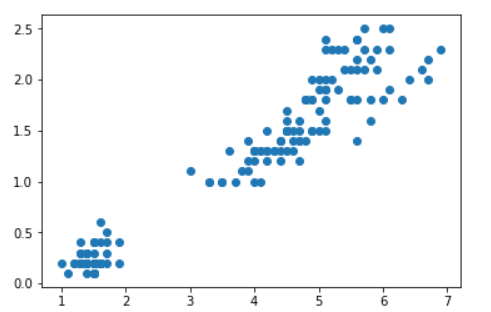
There is a high correlation between the features and the features, so you can take

1) Select one of them
2) Weighted Sum
3) Principal Component Analysis

Feature selection attention!

In all feature selection methods, variance, SelectKBest+various statistics (chi-square filtering, F-test, mutual information), embedding and packaging methods, there is an interface get_support with parameters indices, get_support(indices=False), which can be used to determine which features in the original feature matrix are selected when the parameter is false.Selected, returns the Boolean value True or False, and if indices=True is set, the index of the location of the selected feature in the original feature matrix can be determined.

X_train_columns = X_train.columns
selector = VarianceThreshold(0.005071)
X_fsvar = selector.fit_transform(X_train)
X_fsvar.columns = X_train_columns[selector.get_support(indices=True)]

Dimension Reduction Method 3: Principal Component Analysis (PCA)

Definition: The process of transforming high-dimensional data into status data, in which old data may be discarded and new variables created

Role: Compression of data dimensions, minimizing the dimensionality (complexity) of the original data, and losing a small amount of information

Application: Regression or Classification Analysis

API

sklearn.decomposition.PCA(n_components = None)
    Decomposition data into lower-dimensional spaces

    n_components:
        Decimal: Information indicating how much percent of the package is retained

        Integer: How many features to reduce

    PCA.fit_transform(X)

        Data in X:numpy array format [n_samples, n_features]

        Return: array of specified dimensions after conversion

from sklearn.decomposition import PCA
from sklearn.datasets import load_iris
import pandas as pd

def pca_demo():
    iris = load_iris()
    data = pd.DataFrame(iris.data, columns = iris.feature_names)
    data_array = data.iloc[:, :4].values
    print("data_array:\n", data_array)
    
    transfer = PCA(n_components = 2)
    #ransfer = PCA(n_components = 0.95)
    
    data_pca_value = transfer.fit_transform(data_array)
    print("data_pca_value:\n", data_pca_value)
    
    return None

if __name__ == '__main__':
    pca_demo()




//Output results:
data_array:
 [[5.1 3.5 1.4 0.2]
 [4.9 3.  1.4 0.2]
 [4.7 3.2 1.3 0.2]
 [4.6 3.1 1.5 0.2]
 [5.  3.6 1.4 0.2]
 [5.4 3.9 1.7 0.4]
 [4.6 3.4 1.4 0.3]
 [5.  3.4 1.5 0.2]
 [4.4 2.9 1.4 0.2]
 [4.9 3.1 1.5 0.1]
 [5.4 3.7 1.5 0.2]
 [4.8 3.4 1.6 0.2]
 [4.8 3.  1.4 0.1]
 [4.3 3.  1.1 0.1]
 [5.8 4.  1.2 0.2]
 [5.7 4.4 1.5 0.4]
 [5.4 3.9 1.3 0.4]
 [5.1 3.5 1.4 0.3]
 [5.7 3.8 1.7 0.3]
 [5.1 3.8 1.5 0.3]
 [5.4 3.4 1.7 0.2]
 [5.1 3.7 1.5 0.4]
 [4.6 3.6 1.  0.2]
 [5.1 3.3 1.7 0.5]
 [4.8 3.4 1.9 0.2]
 [5.  3.  1.6 0.2]
 [5.  3.4 1.6 0.4]
 [5.2 3.5 1.5 0.2]
 [5.2 3.4 1.4 0.2]
 [4.7 3.2 1.6 0.2]
 [4.8 3.1 1.6 0.2]
 [5.4 3.4 1.5 0.4]
 [5.2 4.1 1.5 0.1]
 [5.5 4.2 1.4 0.2]
 [4.9 3.1 1.5 0.1]
 [5.  3.2 1.2 0.2]
 [5.5 3.5 1.3 0.2]
 [4.9 3.1 1.5 0.1]
 [4.4 3.  1.3 0.2]
 [5.1 3.4 1.5 0.2]
 [5.  3.5 1.3 0.3]
 [4.5 2.3 1.3 0.3]
 [4.4 3.2 1.3 0.2]
 [5.  3.5 1.6 0.6]
 [5.1 3.8 1.9 0.4]
 [4.8 3.  1.4 0.3]
 [5.1 3.8 1.6 0.2]
 [4.6 3.2 1.4 0.2]
 [5.3 3.7 1.5 0.2]
 [5.  3.3 1.4 0.2]
 [7.  3.2 4.7 1.4]
 [6.4 3.2 4.5 1.5]
 [6.9 3.1 4.9 1.5]
 [5.5 2.3 4.  1.3]
 [6.5 2.8 4.6 1.5]
 [5.7 2.8 4.5 1.3]
 [6.3 3.3 4.7 1.6]
 [4.9 2.4 3.3 1. ]
 [6.6 2.9 4.6 1.3]
 [5.2 2.7 3.9 1.4]
 [5.  2.  3.5 1. ]
 [5.9 3.  4.2 1.5]
 [6.  2.2 4.  1. ]
 [6.1 2.9 4.7 1.4]
 [5.6 2.9 3.6 1.3]
 [6.7 3.1 4.4 1.4]
 [5.6 3.  4.5 1.5]
 [5.8 2.7 4.1 1. ]
 [6.2 2.2 4.5 1.5]
 [5.6 2.5 3.9 1.1]
 [5.9 3.2 4.8 1.8]
 [6.1 2.8 4.  1.3]
 [6.3 2.5 4.9 1.5]
 [6.1 2.8 4.7 1.2]
 [6.4 2.9 4.3 1.3]
 [6.6 3.  4.4 1.4]
 [6.8 2.8 4.8 1.4]
 [6.7 3.  5.  1.7]
 [6.  2.9 4.5 1.5]
 [5.7 2.6 3.5 1. ]
 [5.5 2.4 3.8 1.1]
 [5.5 2.4 3.7 1. ]
 [5.8 2.7 3.9 1.2]
 [6.  2.7 5.1 1.6]
 [5.4 3.  4.5 1.5]
 [6.  3.4 4.5 1.6]
 [6.7 3.1 4.7 1.5]
 [6.3 2.3 4.4 1.3]
 [5.6 3.  4.1 1.3]
 [5.5 2.5 4.  1.3]
 [5.5 2.6 4.4 1.2]
 [6.1 3.  4.6 1.4]
 [5.8 2.6 4.  1.2]
 [5.  2.3 3.3 1. ]
 [5.6 2.7 4.2 1.3]
 [5.7 3.  4.2 1.2]
 [5.7 2.9 4.2 1.3]
 [6.2 2.9 4.3 1.3]
 [5.1 2.5 3.  1.1]
 [5.7 2.8 4.1 1.3]
 [6.3 3.3 6.  2.5]
 [5.8 2.7 5.1 1.9]
 [7.1 3.  5.9 2.1]
 [6.3 2.9 5.6 1.8]
 [6.5 3.  5.8 2.2]
 [7.6 3.  6.6 2.1]
 [4.9 2.5 4.5 1.7]
 [7.3 2.9 6.3 1.8]
 [6.7 2.5 5.8 1.8]
 [7.2 3.6 6.1 2.5]
 [6.5 3.2 5.1 2. ]
 [6.4 2.7 5.3 1.9]
 [6.8 3.  5.5 2.1]
 [5.7 2.5 5.  2. ]
 [5.8 2.8 5.1 2.4]
 [6.4 3.2 5.3 2.3]
 [6.5 3.  5.5 1.8]
 [7.7 3.8 6.7 2.2]
 [7.7 2.6 6.9 2.3]
 [6.  2.2 5.  1.5]
 [6.9 3.2 5.7 2.3]
 [5.6 2.8 4.9 2. ]
 [7.7 2.8 6.7 2. ]
 [6.3 2.7 4.9 1.8]
 [6.7 3.3 5.7 2.1]
 [7.2 3.2 6.  1.8]
 [6.2 2.8 4.8 1.8]
 [6.1 3.  4.9 1.8]
 [6.4 2.8 5.6 2.1]
 [7.2 3.  5.8 1.6]
 [7.4 2.8 6.1 1.9]
 [7.9 3.8 6.4 2. ]
 [6.4 2.8 5.6 2.2]
 [6.3 2.8 5.1 1.5]
 [6.1 2.6 5.6 1.4]
 [7.7 3.  6.1 2.3]
 [6.3 3.4 5.6 2.4]
 [6.4 3.1 5.5 1.8]
 [6.  3.  4.8 1.8]
 [6.9 3.1 5.4 2.1]
 [6.7 3.1 5.6 2.4]
 [6.9 3.1 5.1 2.3]
 [5.8 2.7 5.1 1.9]
 [6.8 3.2 5.9 2.3]
 [6.7 3.3 5.7 2.5]
 [6.7 3.  5.2 2.3]
 [6.3 2.5 5.  1.9]
 [6.5 3.  5.2 2. ]
 [6.2 3.4 5.4 2.3]
 [5.9 3.  5.1 1.8]]
data_pca_value:
 [[-2.68420713  0.32660731]
 [-2.71539062 -0.16955685]
 [-2.88981954 -0.13734561]
 [-2.7464372  -0.31112432]
 [-2.72859298  0.33392456]
 [-2.27989736  0.74778271]
 [-2.82089068 -0.08210451]
 [-2.62648199  0.17040535]
 [-2.88795857 -0.57079803]
 [-2.67384469 -0.1066917 ]
 [-2.50652679  0.65193501]
 [-2.61314272  0.02152063]
 [-2.78743398 -0.22774019]
 [-3.22520045 -0.50327991]
 [-2.64354322  1.1861949 ]
 [-2.38386932  1.34475434]
 [-2.6225262   0.81808967]
 [-2.64832273  0.31913667]
 [-2.19907796  0.87924409]
 [-2.58734619  0.52047364]
 [-2.3105317   0.39786782]
 [-2.54323491  0.44003175]
 [-3.21585769  0.14161557]
 [-2.30312854  0.10552268]
 [-2.35617109 -0.03120959]
 [-2.50791723 -0.13905634]
 [-2.469056    0.13788731]
 [-2.56239095  0.37468456]
 [-2.63982127  0.31929007]
 [-2.63284791 -0.19007583]
 [-2.58846205 -0.19739308]
 [-2.41007734  0.41808001]
 [-2.64763667  0.81998263]
 [-2.59715948  1.10002193]
 [-2.67384469 -0.1066917 ]
 [-2.86699985  0.0771931 ]
 [-2.62522846  0.60680001]
 [-2.67384469 -0.1066917 ]
 [-2.98184266 -0.48025005]
 [-2.59032303  0.23605934]
 [-2.77013891  0.27105942]
 [-2.85221108 -0.93286537]
 [-2.99829644 -0.33430757]
 [-2.4055141   0.19591726]
 [-2.20883295  0.44269603]
 [-2.71566519 -0.24268148]
 [-2.53757337  0.51036755]
 [-2.8403213  -0.22057634]
 [-2.54268576  0.58628103]
 [-2.70391231  0.11501085]
 [ 1.28479459  0.68543919]
 [ 0.93241075  0.31919809]
 [ 1.46406132  0.50418983]
 [ 0.18096721 -0.82560394]
 [ 1.08713449  0.07539039]
 [ 0.64043675 -0.41732348]
 [ 1.09522371  0.28389121]
 [-0.75146714 -1.00110751]
 [ 1.04329778  0.22895691]
 [-0.01019007 -0.72057487]
 [-0.5110862  -1.26249195]
 [ 0.51109806 -0.10228411]
 [ 0.26233576 -0.5478933 ]
 [ 0.98404455 -0.12436042]
 [-0.174864   -0.25181557]
 [ 0.92757294  0.46823621]
 [ 0.65959279 -0.35197629]
 [ 0.23454059 -0.33192183]
 [ 0.94236171 -0.54182226]
 [ 0.0432464  -0.58148945]
 [ 1.11624072 -0.08421401]
 [ 0.35678657 -0.06682383]
 [ 1.29646885 -0.32756152]
 [ 0.92050265 -0.18239036]
 [ 0.71400821  0.15037915]
 [ 0.89964086  0.32961098]
 [ 1.33104142  0.24466952]
 [ 1.55739627  0.26739258]
 [ 0.81245555 -0.16233157]
 [-0.30733476 -0.36508661]
 [-0.07034289 -0.70253793]
 [-0.19188449 -0.67749054]
 [ 0.13499495 -0.31170964]
 [ 1.37873698 -0.42120514]
 [ 0.58727485 -0.48328427]
 [ 0.8072055   0.19505396]
 [ 1.22042897  0.40803534]
 [ 0.81286779 -0.370679  ]
 [ 0.24519516 -0.26672804]
 [ 0.16451343 -0.67966147]
 [ 0.46303099 -0.66952655]
 [ 0.89016045 -0.03381244]
 [ 0.22887905 -0.40225762]
 [-0.70708128 -1.00842476]
 [ 0.35553304 -0.50321849]
 [ 0.33112695 -0.21118014]
 [ 0.37523823 -0.29162202]
 [ 0.64169028  0.01907118]
 [-0.90846333 -0.75156873]
 [ 0.29780791 -0.34701652]
 [ 2.53172698 -0.01184224]
 [ 1.41407223 -0.57492506]
 [ 2.61648461  0.34193529]
 [ 1.97081495 -0.18112569]
 [ 2.34975798 -0.04188255]
 [ 3.39687992  0.54716805]
 [ 0.51938325 -1.19135169]
 [ 2.9320051   0.35237701]
 [ 2.31967279 -0.24554817]
 [ 2.91813423  0.78038063]
 [ 1.66193495  0.2420384 ]
 [ 1.80234045 -0.21615461]
 [ 2.16537886  0.21528028]
 [ 1.34459422 -0.77641543]
 [ 1.5852673  -0.53930705]
 [ 1.90474358  0.11881899]
 [ 1.94924878  0.04073026]
 [ 3.48876538  1.17154454]
 [ 3.79468686  0.25326557]
 [ 1.29832982 -0.76101394]
 [ 2.42816726  0.37678197]
 [ 1.19809737 -0.60557896]
 [ 3.49926548  0.45677347]
 [ 1.38766825 -0.20403099]
 [ 2.27585365  0.33338653]
 [ 2.61419383  0.55836695]
 [ 1.25762518 -0.179137  ]
 [ 1.29066965 -0.11642525]
 [ 2.12285398 -0.21085488]
 [ 2.3875644   0.46251925]
 [ 2.84096093  0.37274259]
 [ 3.2323429   1.37052404]
 [ 2.15873837 -0.21832553]
 [ 1.4431026  -0.14380129]
 [ 1.77964011 -0.50146479]
 [ 3.07652162  0.68576444]
 [ 2.14498686  0.13890661]
 [ 1.90486293  0.04804751]
 [ 1.16885347 -0.1645025 ]
 [ 2.10765373  0.37148225]
 [ 2.31430339  0.18260885]
 [ 1.92245088  0.40927118]
 [ 1.41407223 -0.57492506]
 [ 2.56332271  0.2759745 ]
 [ 2.41939122  0.30350394]
 [ 1.94401705  0.18741522]
 [ 1.52566363 -0.37502085]
 [ 1.76404594  0.07851919]
 [ 1.90162908  0.11587675]
 [ 1.38966613 -0.28288671]]




Reference link: https://www.cnblogs.com/ftl1012/p/10498480.html

Posted by drummer101 on Fri, 27 Sep 2019 23:41:55 -0700

Programmer Group

Three ways of feature dimension reduction

Two ways to reduce dimensions:

1. Feature Selection

2. Principal Component Analysis (can be understood as a feature extraction method)

1. Feature Selection

2 methods for feature selection (filter + embedded)

Modular

1. Dimension Reduction Method 1: Feature Selection - Filtering - Low Variance Filtering

Low variance feature filtering

API

Dimension reduction method 2: feature selection - Filter - correlation coefficient

API

There is a high correlation between the features and the features, so you can take

Feature selection attention!

Dimension Reduction Method 3: Principal Component Analysis (PCA)

API

Hot Keywords