RNN principle
-
Cyclic neural network: processing sequence model, weight sharing.
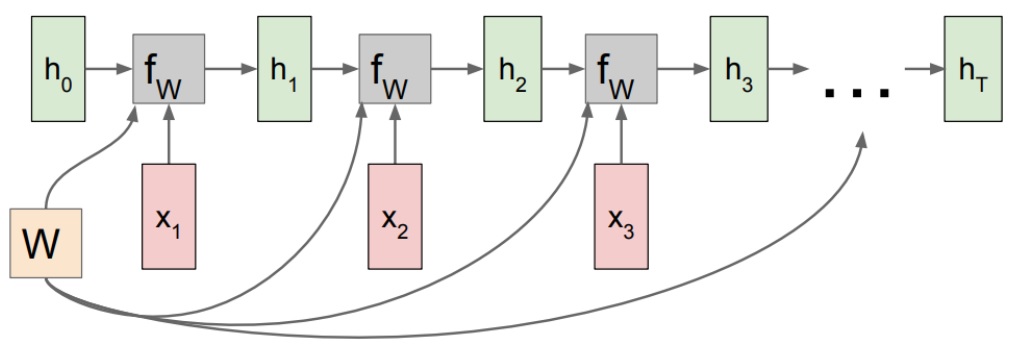
h[t] = fw(h[t-1], x[t])	#fw is some function with parameters W
h[t] = tanh(W[h,h]*h[t-1] + W[x,h]*x[t])    #to be specific
y[t] = W[h,y]*h[t]
-
Sequence to Sequence model

-
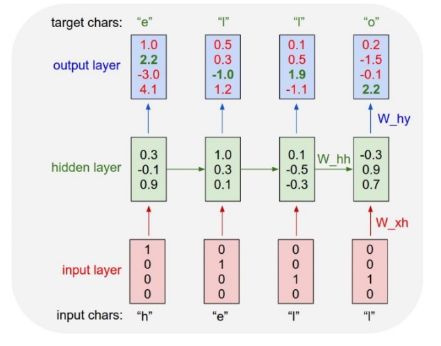
Schematic diagram of language model
RNN actual combat
-
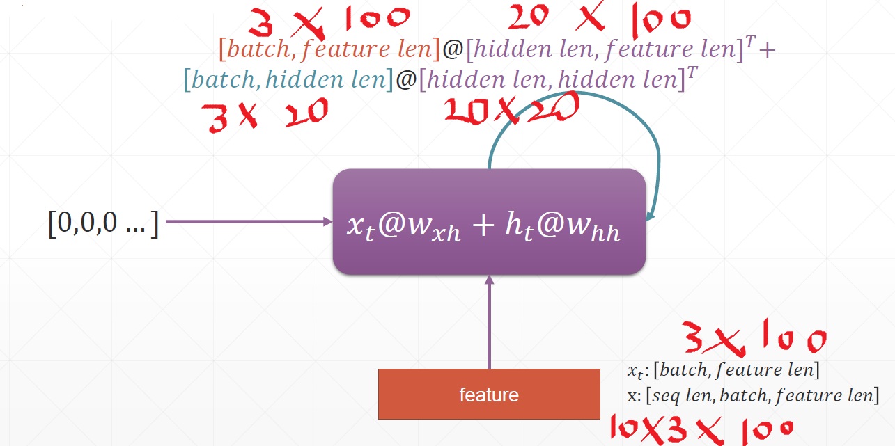
Three sentences, one sentence 10 words, one word 100 dimensions
-
Basic usage
rnn = nn.RNN(100,10)	#input_size(feature_len)=100,hidden_len = 10
rnn._parameters.keys()  #How many sensors (w and B of four l0 layers)

nn.RNN(input_size,hidden_size, num_layers = 1)
#h0 : [layer, batchsz, hidden]  x : [seq, batchsz, input ]
#ht : [layer, batchsz, hidden] out: [seq, batchsz, hidden]
out, ht = forward(x, h0)
#For multilayer rnn, out remains the same (the last mem state at all times), ht becomes [2, ~, ~] (the last time state at all layers)

cell = nn.RNNcell()	#The parameters are the same as nn.RNN(), but xt should be entered for each timestamp
for xt in x:
	h1 = cell(xt,h1)

#If you want to enter x in this format: [batchsz, seq_len, input]
#Need to add parameter in nn.RNN(): batch Ou first = true
-
Building a very simple RNN model (taking a simple time series prediction as an example)
class Net(nn.Module):
	def __init__(self,input_size,hidden_size):
        super(net, self).__init__()
        self.rnn = nn.RNN(
            input_size=input_size,
            hidden_size=hidden_size,
            num_layers=1,
            batch_first=True,
        )
        for p in self.rnn.parameters():#Initialization of weights for normal distribution
            nn.init.normal_(p, mean=0.0, std=0.001)
        self.linear = nn.Linear(hidden_size, output_size)
	def forward(self,x,h0):
    	out, ht = self.rnn(x, h0)	   #out:[batch_sz,seq,hidden_sz]
       	out = out.view(-1, hidden_size)#out:[seq,hidden_size](b=1)
       	out = self.linear(out)		   #out:[seq,output_size]
       	out = out.unsqueeze(dim=0)	   #out:[1,seq,output_size]
       	return out, ht
-
When we calculate the gradient of RNN by back propagation, there is a whhkw {HH} ^ {K} whhk in the final derivative term, which will cause the gradient to explode or disappear.
# Solving gradient explosion
for p in net.parameters():
    torch.nn.utils.clip_grad_norm_(p, 10)	# Ensure that the absolute value of gradient is less than 10
# Solving gradient dispersion: LSTM
-
LSTM: long short term memory (structure as shown in the figure below)
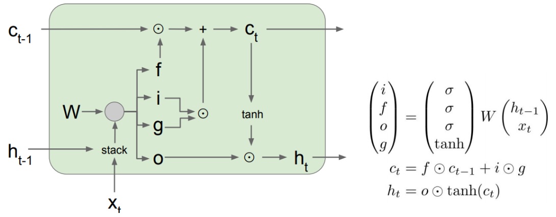
There are three gates: forgetting gate fff, input gate iii and output gate ooo. For input and output variables: ct − 1c {T-1} ct − 1 is the input memory (new, to solve the problem of gradient discretization and enhance memory), XTX ﹣ TXT is the input, ht ﹣ 1H {T-1} ht − 1 is the output of the previous time unit, and CTC {t} ct is the memory transmitted to the next time unit.-
Forgetting gate: f t = σ (Wf × [ht − 1, xt] + B F) f_t = \ sigma (w_f \ times [h {T-1}, X {t}] + b_f) ft = σ (Wf × [ht − 1, xt] + bf)
-
Input gate: I t = σ (Wi × [ht − 1, xt] + B I) i t = \ sigma (w_i \ times [h {T-1}, X {t}] + b_i) it = σ (Wi × [ht − 1, xt] + bi)
-
Output gate: o t = σ (Wo × [ht − 1, xt] + b o) o t = \ sigma (w_o \ times [h {T-1}, X {t}] + b_o) ot = σ (Wo × [ht − 1, xt] + bo)
-
Filter input: c t ~ = tanh(Wc × [ht − 1, xt] + B C) \ widetilde {C} = tanh (w {C \ times [h {T-1}, X {t}] + B  ̄ C) CT = tanh(Wc × [ht − 1, xt] + bc). The result is filtered input
Then, the new memory is equal to "the previous memory retained after the forgetting gate acts" + "the new filtered input retained after the input gate acts", that is, c t = ft × ct − 1+it × ct ~ C t = f t \ times C {T-1} + I t \ times \ widetime {C t} ct=ft × ct − 1+it × ct. The new output (h) is equal t o the "new memory processed by tanh" retained after the action of the output gate, that is, h t = ot × tanh(ct) H ﹐ t = O ﹐ t \ times tanh (C ﹐ T) ht=ot × tanh(ct).
-
-
LSTM layer
# initial
nn.LSTM(input_size,hidden_size, num_layers = 1)
# forward
#   x : [seq, batchsz, input]    out : [seq, batchsz, hidden]
# h/c : [layer, batchsz, hidden]
out, (ht, ct) = lstm(x, [h0, c0])

# silimar to LSTMcell
cell = nn.LSTMcell(~)
for xt in x:
    h, c = cell(xt, [h, c])
The practical battle of emotion classification
-
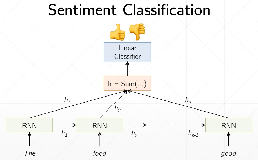
Taobao, for example, classifies good reviews and bad reviews. The model is as follows. After embedding each word, it is sent to RNN, and emotion categories are synthesized for all outputs.
-
Load data set (very important package)
from torchtext import data, datasets
# data.Field(): the string is split on the space by default, and the token is set to spacy for English word segmentation
#				 Processing methods used to define fields
TEXT = data.Field(tokenize='spacy')
# LabelField is a subclass of Field, which is specially used to handle labels
LABEL = data.LabelField(dtype=torch.float)
# Load IMDB movie review dataset
train_data, test_data = datasets.IMDB.splits(TEXT, LABEL)
-
We use Glove word vector model to build corpus, and batch the processed data. The function of bucket iterator is to divide several batches according to the similar length, and each batch is supplemented with corresponding length.
TEXT.build_vocab(train_data,max_size=10000,vectors='glove.6B.100d')
LABEL.build_vocab(train_data)
train_iterator, test_iterator = data.BucketIterator.splits(
    (train_data, test_data),
    batch_size = batchsz,
    device=device
)
-
network structure
class LSTM_Net(nn.Module):
    def __init__(self, vocab_size, embedding_dim, hidden_dim):
        super(LSTM_Net, self).__init__()
        # [0-10001] => [100] [vb -> embedding]
        self.embedding = nn.Embedding(vocab_size, embedding_dim)
        # [100] => [256] [embedding -> hidden]
        self.lstm = nn.LSTM(embedding_dim, hidden_dim, num_layers=2,
                           bidirectional=True, dropout=0.5)
        # [256*2] => [1]
        self.fc = nn.Linear(hidden_dim*2, 1)
        self.dropout = nn.Dropout(0.5)
    def forward(self, x):
        # [SEQ, batchsz, 1 (string)] = > [SEQ, batchsz, 100]
        embedding = self.dropout(self.embedding(x))
        # output: [seq, batchsz, hidden*2] because it's double-layer
        # hidden/cell: [layers, batchsz, hidden]
        # hidden is the output of each timestamp
        output, (hidden, cell) = self.lstm(embedding)
        # [layers*2, batchsz, hidden] => [batchsz, hidden*2]
        # torch.cat(): splice the first two torches by dimension 1
        hidden = torch.cat([hidden[-2], hidden[-1]], dim=1)
        # [batchsz, hidden*2] => [b, 1]
        hidden = self.dropout(hidden)
        out = self.fc(hidden)
        return out
-
Embedding initialization
rnn = LSTM_Net(len(TEXT.vocab), 100, 256)
pretrained_embedding = TEXT.vocab.vectors 	# Specify the initial weight (obtained by glove)
rnn.embedding.weight.data.copy_(pretrained_embedding)# Import initialization weights
-
Define optimizer and loss function
optimizer = optim.Adam(rnn.parameters(), lr=1e-3)
criteon = nn.BCEWithLogitsLoss()	# Two class cross entropy loss function
-
Training and testing
def binary_acc(preds, y):
    preds = torch.round(torch.sigmoid(preds))
    correct = torch.eq(preds, y).float()
    acc = correct.sum() / len(correct)
    return acc

def train(rnn, iterator, optimizer, criteon):
    avg_acc = []
    lstm.train()
    for i, batch in enumerate(iterator):
        # [seq, b] => [b, 1] => [b]
        pred = lstm(batch.text).squeeze(1)
        loss = criteon(pred, batch.label)
        acc = binary_acc(pred, batch.label).item()
        avg_acc.append(acc)

        optimizer.zero_grad()
        loss.backward()
        optimizer.step()
    avg_acc = np.array(avg_acc).mean()
    print('train acc:', avg_acc)


def eval(rnn, iterator, criteon):
    avg_acc = []
    lstm.eval()
    with torch.no_grad():
        for batch in iterator:
            # [b, 1] => [b]
            pred = lstm(batch.text).squeeze(1)
            loss = criteon(pred, batch.label)
            acc = binary_acc(pred, batch.label).item()
            avg_acc.append(acc)
    avg_acc = np.array(avg_acc).mean()
    print('test acc:', avg_acc)

