[introduction]: in the previous article about IIR design, some friends are still reading it. Although I don't know how the officials feel, I think there is always a reward to read, so I decided to continue this series. This article talks about average filter, which is very easy at first glance. But I don't think some of the key points are clear. This paper focuses on the internal mechanism and application scenarios of xx one-dimensional average filter design.
Note: try to write a summary in each article for easy reading. In the information age, everyone's time is precious, which can also save fans' precious time.
Theoretical understanding
To learn one thing, personal advice should be carried out from three dimensions: what how
The content here mainly refers to the introduction to digital signal processing written by Hu Guangshu 7.5.1 Section, added some of their own understanding.
When it comes to average filter, a friend who has done the application and development of single-chip microcomputer can immediately think of adding and averaging some sampling data. It is true that the mathematical description of the time domain is also intuitive:
Where \ (x(n) \) represents the current measurement value. For SCM applications, it can be the sampling value of the current ADC or the physical quantity of the current sensor after a series of processing (such as the temperature, pressure, flow and other measurement values in the industrial control field), while \ (x(n-1) \) represents the last measurement value, and so on, \ (x(n-N+1) \) is the previous N-1 measurement value.
In order to reveal its deeper mechanism, the above formula is further described by Z transfer function:
For Fourier transform:
The essence of Z-transform is the discretization form of Laplacian transform, \ (Z=e^{\sigma+j\omega}=e^{\sigma}e^{j\omega} \), let \ (e^{\sigma}=r \), then
Let \ (r=1 \), then
Therefore, the frequency response of the average filter is:
Amplitude frequency phase frequency analysis
Use the following python code to analyze
# encoding: UTF-8
from scipy.optimize import newton
from scipy.signal import freqz, dimpulse, dstep
from math import sin, cos, sqrt, pi
import numpy as np
import matplotlib.pyplot as plt
import sys
reload(sys)
sys.setdefaultencoding('utf8')

#Function used to calculate cut-off frequency of moving average filter
def get_filter_cutoff(N, **kwargs):
    func = lambda w: sin(N*w/2) - N/sqrt(2) * sin(w/2)
    deriv = lambda w: cos(N*w/2) * N/2 - N/sqrt(2) * cos(w/2) / 2
    omega_0 = pi/N  # Starting condition: halfway the first period of sin
    return newton(func, omega_0, deriv, **kwargs)

#Set sample rate
sample_rate = 200 #Hz
N = 7


# Calculate cut-off frequency
w_c = get_filter_cutoff(N)
cutoff_freq = w_c * sample_rate / (2 * pi)

# Filter parameters
b = np.ones(N)
a = np.array([N] + [0]*(N-1))

#frequency response
w, h = freqz(b, a, worN=4096)
#Turn to frequency
w *= sample_rate / (2 * pi)

#Draw bode map
plt.subplot(2, 1, 1)
plt.suptitle("Bode")
#Convert to decibels
plt.plot(w, 20 * np.log10(abs(h)))
plt.ylabel('Magnitude [dB]')
plt.xlim(0, sample_rate / 2)
plt.ylim(-60, 10)
plt.axvline(cutoff_freq, color='red')
plt.axhline(-3.01, linewidth=0.8, color='black', linestyle=':')

# Phase frequency response
plt.subplot(2, 1, 2)
plt.plot(w, 180 * np.angle(h) / pi)
plt.xlabel('Frequency [Hz]')
plt.ylabel('Phase [°]')
plt.xlim(0, sample_rate / 2)
plt.ylim(-180, 90)
plt.yticks([-180, -135, -90, -45, 0, 45, 90])
plt.axvline(cutoff_freq, color='red')
plt.show()
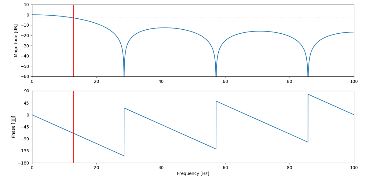
If the sampling rate is 200Hz and the filter length is 7, the following amplitude frequency and phase frequency response curves can be obtained. It can be seen from its main lobe that its amplitude frequency response is a low-pass filter. The amplitude frequency response is slightly uneven and attenuates with the increase of frequency. Its phase frequency response is linear. If you have experience in FIR filter, you will know that the phase frequency response of FIR filter is linear, and the moving average filter is just a special case of fir.
When the filter length is changed to 3 / 7 / 21, only the amplitude frequency response is observed:
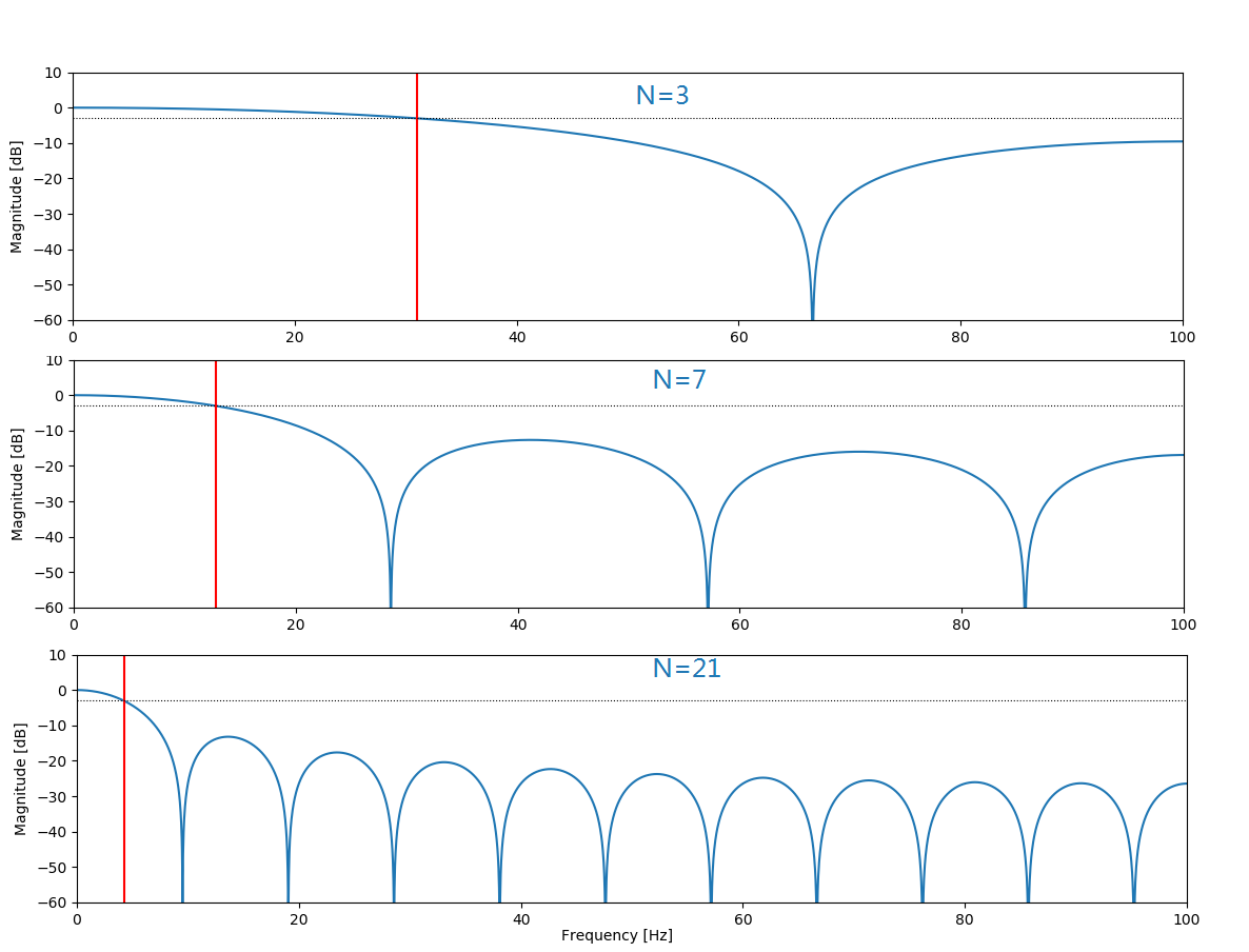
It can be seen that as the length of the filter becomes longer, its cut-off frequency becomes smaller and its passband becomes narrower. The response of the filter is slower and the delay is larger. Therefore, the length of the filter must be reasonably selected according to the useful frequency bandwidth in actual use. The bandwidth of useful signal can be obtained by Fourier analysis by collecting certain points according to sampling rate. If there is an oscilloscope with FFT function, it can also be measured directly.
C realization of filter
It is easy to implement the filter in C language. Share the code here:
#define MVF_LENGTH  5
typedef float E_SAMPLE;
/*Define moving average register history status*/
typedef struct  _t_MAF
{
    E_SAMPLE buffer[MVF_LENGTH];
    E_SAMPLE sum;
    int index;
}t_MAF;

void moving_average_filter_init(t_MAF * pMaf)
{
    pMaf->index = -1;
    pMaf->sum   = 0;
}

E_SAMPLE moving_average_filter(t_MAF * pMaf,E_SAMPLE xn)
{
    E_SAMPLE yn=0;
    int i=0;

    if(pMaf->index == -1)
    {
        for(i = 0; i < MVF_LENGTH; i++)
        {
            pMaf->buffer[i] = xn;
        }
        pMaf->sum   = xn*MVF_LENGTH;
        pMaf->index = 0;
    }
    else
    {
        if(xn>100)
            xn = xn+0.1;
        pMaf->sum     -= pMaf->buffer[pMaf->index];
        pMaf->buffer[pMaf->index] = xn;
        pMaf->sum     += xn;
        pMaf->index++;
        if(pMaf->index>=MVF_LENGTH)
            pMaf->index = 0;
    }
    yn = pMaf->sum/MVF_LENGTH;
    return yn;
}
Test code:
#define SAMPLE_RATE 500.0f
#define SAMPLE_SIZE 256
#define PI 3.415926f
int main()
{
    E_SAMPLE rawSin[SAMPLE_SIZE];
    E_SAMPLE outSin[SAMPLE_SIZE];

    E_SAMPLE rawSquare[SAMPLE_SIZE];
    E_SAMPLE outSquare[SAMPLE_SIZE];
    t_MAF mvf;

    FILE *pFile=fopen("./simulationSin.csv","wt+");
    /*Sine signal test*/
    if(pFile==NULL)
    {
        printf("simulationSin.csv opened failed");
        return -1;
    }
    for(int i=0;i<SAMPLE_SIZE;i++)
    {
        rawSin[i] = 100*sin(2*PI*20*i/SAMPLE_RATE)+rand()%30;
    }

    /*Square wave test*/
    for(int i=0;i<SAMPLE_SIZE/4;i++)
    {
        rawSquare[i] = 5+rand()%10;
    }
    for(int i=SAMPLE_SIZE/4;i<3*SAMPLE_SIZE/4;i++)
    {
        rawSquare[i] = 100+rand()%10;
    }
    for(int i=3*SAMPLE_SIZE/4;i<SAMPLE_SIZE;i++)
    {
        rawSquare[i] = 5+rand()%10;
    }

    /*initialization*/
    moving_average_filter_init(&mvf);
    /*wave filtering*/
    for(int i=0;i<SAMPLE_SIZE;i++)
    {
        outSin[i]=moving_average_filter(&mvf,rawSin[i]);
    }

    for(int i=0;i<SAMPLE_SIZE;i++)
    {
        fprintf(pFile,"%f,",rawSin[i]);
    }

    fprintf(pFile,"\n");
    for(int i=0;i<SAMPLE_SIZE;i++)
    {
        fprintf(pFile,"%f,",outSin[i]);
    }

    fclose(pFile);

    pFile=fopen("./simulationSquare.csv","wt+");
    if(pFile==NULL)
    {
        printf("simulationSquare.csv opened failed");
        return -1;
    }
    /*initialization*/
    moving_average_filter_init(&mvf);
    /*wave filtering*/
    for(int i=0;i<SAMPLE_SIZE;i++)
    {
        outSquare[i]=moving_average_filter(&mvf,rawSquare[i]);
    }

    for(int i=0;i<SAMPLE_SIZE;i++)
    {
        fprintf(pFile,"%f,",rawSquare[i]);
    }

    fprintf(pFile,"\n");
    for(int i=0;i<SAMPLE_SIZE;i++)
    {
        fprintf(pFile,"%f,",outSquare[i]);
    }

    fclose(pFile);
    return 0;
}
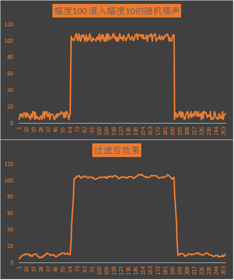
For square wave test, the following waveforms can be obtained by using excel to generate waveforms. It can be seen from the waveform that the moving average filter with length of 7 is quite satisfied with the filtering effect of random noise. It can also be seen from the figure that the moving average filter will introduce a certain delay in the signal chain, which needs to be considered in the application. If there is no clear requirement for general sensor measurement, it can often be ignored.
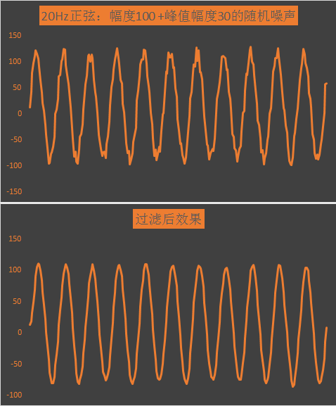
For sinusoidal signal, the moving average filter also has obvious effect, but its passband is narrow. If the useful signal frequency is high, the moving average filter will not be suitable.
Summary:
- The moving average filter has a good effect in removing high frequency noise.
- Moving average filter is essentially a FIR filter, which has a linear phase frequency response.
- In practical use, it is necessary to pay attention to the useful signal frequency. If the useful signal frequency is high, it is not applicable.
- The length should not be too long, or its delay effect will be great.
- From the point of view of the signal chain, it can be used as the pre-processing, that is, the direct filtering of the data after the ADC. It can also be used as a post-processing.
- If it is ADC sampling data filtering and the sample is integer, the code in this paper can be optimized accordingly. For example, multiplication division can be replaced by shift left and shift right.
The article is from WeChat official account: embedded Inn, focusing on official account, and getting more updates.