But I found that this method would change the amplitude of the signal. N-fold interpolation reduces the amplitude by n-fold. Therefore, the third step should be added: n times the amplitude of the signal after filtering multiplied by n.

import numpy as np
import math
import scipy.signal as signal
import pylab as pl
import matplotlib.pyplot as plt

sampling_rate=1000 # The sampling rate is set to 1000Hz, and the sampling rate before interpolation is 333Hz
t1=np.arange(0, 1.0, 1.0/sampling_rate) # Time length is 1s
x1=np.sin(15.4*np.pi*t1)*8.9+np.sin(31*np.pi*t1)*35.9+np.sin(56*np.pi*t1)*29.3
plt.figure(figsize=(16,4))
plt.plot(t1,x1)
plt.plot(t1,x1, '*')
plt.xlabel("Time(s)")
plt.ylabel("Volt")
plt.legend()
plt.show()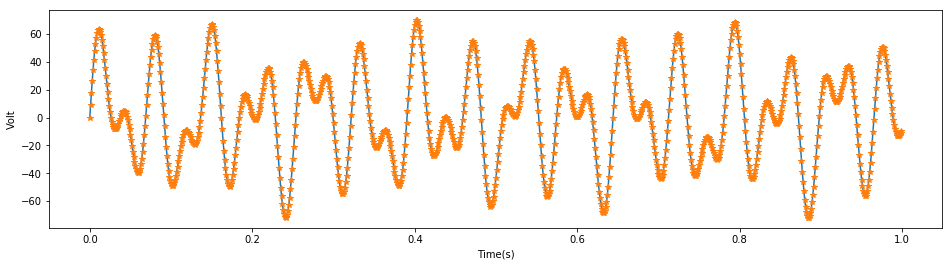

# x2 is the data before interpolation
t2=t1[::3]
x2=x1[::3]
plt.figure(figsize=(16,4))
plt.plot(t2,x2,"*")
plt.plot(t2,x2)
plt.xlabel("Time(s)")
plt.ylabel("Volt")
plt.legend()
plt.show()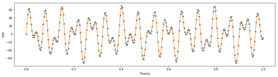

# x3 is zero value interpolation modified digital signal
x3=x1.copy()
x3[1::3]=0;
x3[2::3]=0;
plt.figure(figsize=(16,4))
plt.plot(t1,x3,"*")
plt.xlabel("Time(s)")
plt.ylabel("Volt")
plt.legend()
plt.show()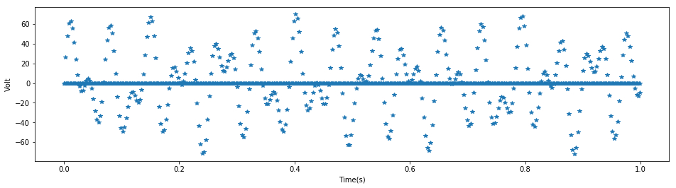

# Amplify local signal
plt.figure(figsize=(16,4))
plt.plot(t1,x3,"*")
plt.xlim(0,0.1)
plt.xlabel("Time(s)")
plt.ylabel("Volt")
plt.legend()
plt.show()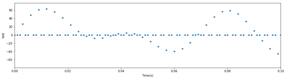

# Filter settings
b,a=signal.iirdesign(0.08, 0.1, 1, 40)
# x4 is the digital signal filtered by low-pass filter
x4 = signal.filtfilt(b, a, x3)
plt.figure(figsize=(16,4))
plt.plot(t1,x4)
plt.plot(t1,x4,"*")
plt.xlabel("Time(s)")
plt.ylabel("Volt")
plt.legend()
plt.show()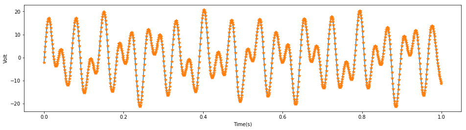

# Blue is the theoretical signal and red is the signal after the first two steps of interpolation
plt.figure(figsize=(16,4))
plt.plot(t1,x1)
plt.plot(t1,x4,'r--')
plt.xlabel("Time(s)")
plt.ylabel("Volt")
plt.legend()
plt.show()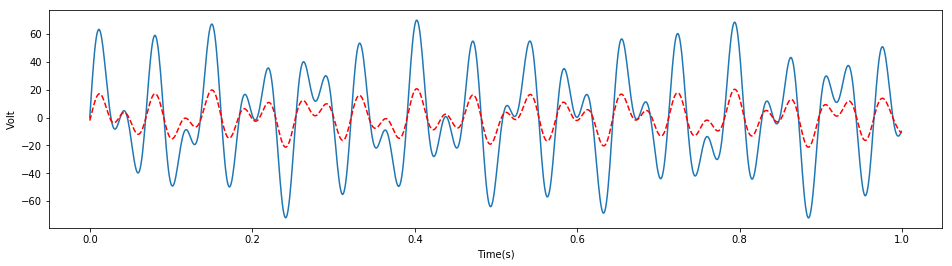

It can be seen that the signal amplitude after filtering has been changed to a large extent.

# Blue is the theoretical signal and red is the interpolated signal
plt.figure(figsize=(16,4))
plt.plot(t1,x1)
plt.plot(t1,3*x4,'r--')
plt.xlabel("Time(s)")
plt.ylabel("Volt")
plt.legend()
plt.show()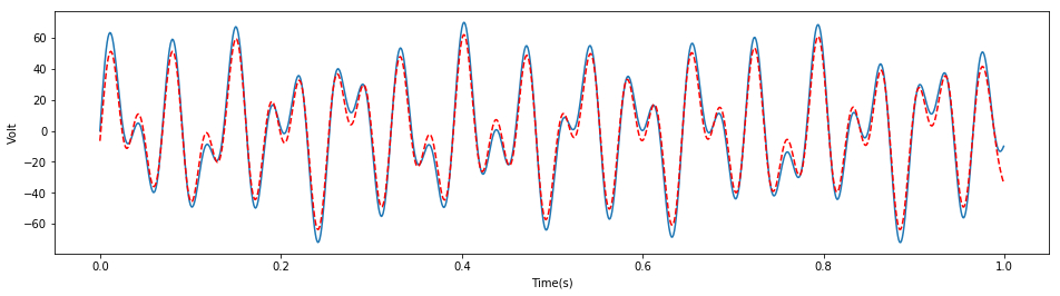

Conclusion:
The zero value interpolation method of signal needs three steps:
1. Insert the zero value sample (i.e. insert 0 where interpolation is needed)
2. Low pass filter filtering
3. For n times interpolation, each signal value is increased by n times