1. FCN full convolution neural network for semantic segmentation

Long J , Shelhamer E , Darrell T . Fully Convolutional Networks for Semantic Segmentation[J]. IEEE Transactions on Pattern Analysis & Machine Intelligence, 2014, 39(4):640-651.

                    

• Loss of image details during down sampling
• The contradiction between image semantic information and location information

                         .

Specifically, in the process of down sampling, the size of the feature image is decreasing, which inevitably discards some information, which is usually the location information of the target in the image.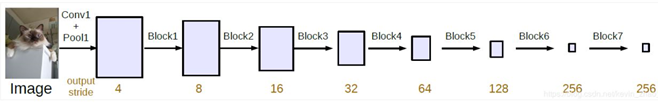

Why do you need to take samples? Because this is the requirement for the classification of objects in the image. For example, the typical image classification network VGG-16 shown in the figure below, after the full connection layer, becomes a vector of (1000,1), indicating the probability of belonging to each category.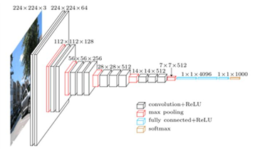

                               .

Based on the two contradictory problems of semantic segmentation, FCN proposes to use full convolution and jump structure.

                                    There are various adjustments and improvements.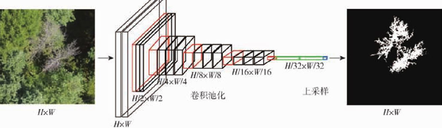

The second feature of    model is the jump structure. According to the feature maps of different sizes generated by the full winder network above, the feature maps generated by different layers are selected for up sampling and fusion, as shown in the following figure: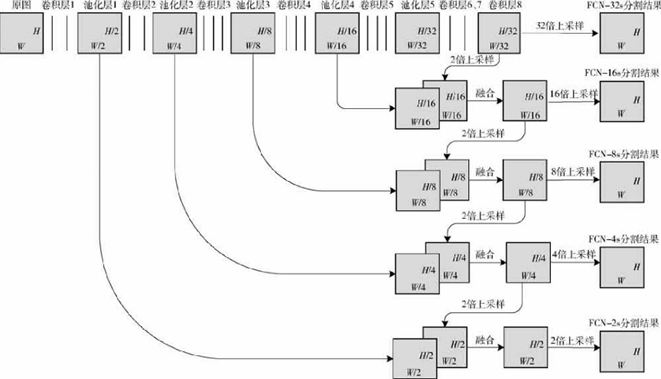

Based on this jump structure, there are FCN-32s (32x up sampling as segmentation result), FCN-16s (32x up sampling as segmentation result), FCN-8s, and even FCN-4s and FCN-2s.

   take FCN-16s as an example to briefly look at the code:

class FCN16s(nn.Module):
    def __init__(self, pretrained_net, n_class):
        super().__init__()
        self.n_class = n_class
        self.pretrained_net = pretrained_net
        self.relu    = nn.ReLU(inplace=True)
        self.deconv1 = nn.ConvTranspose2d(512, 512, kernel_size=3, stride=2, padding=1, dilation=1, output_padding=1)
        self.bn1     = nn.BatchNorm2d(512)
        self.deconv2 = nn.ConvTranspose2d(512, 256, kernel_size=3, stride=2, padding=1, dilation=1, output_padding=1)
        self.bn2     = nn.BatchNorm2d(256)
        self.deconv3 = nn.ConvTranspose2d(256, 128, kernel_size=3, stride=2, padding=1, dilation=1, output_padding=1)
        self.bn3     = nn.BatchNorm2d(128)
        self.deconv4 = nn.ConvTranspose2d(128, 64, kernel_size=3, stride=2, padding=1, dilation=1, output_padding=1)
        self.bn4     = nn.BatchNorm2d(64)
        self.deconv5 = nn.ConvTranspose2d(64, 32, kernel_size=3, stride=2, padding=1, dilation=1, output_padding=1)
        self.bn5     = nn.BatchNorm2d(32)
        self.classifier = nn.Conv2d(32, n_class, kernel_size=1)

    def forward(self, x):
        output = self.pretrained_net(x)
        x5 = output['x5']  # size=(N, 512, x.H/32, x.W/32)
        x4 = output['x4']  # size=(N, 512, x.H/16, x.W/16)

        score = self.relu(self.deconv1(x5))               # size=(N, 512, x.H/16, x.W/16)
        score = self.bn1(score + x4)                      # element-wise add, size=(N, 512, x.H/16, x.W/16)
        score = self.bn2(self.relu(self.deconv2(score)))  # size=(N, 256, x.H/8, x.W/8)
        score = self.bn3(self.relu(self.deconv3(score)))  # size=(N, 128, x.H/4, x.W/4)
        score = self.bn4(self.relu(self.deconv4(score)))  # size=(N, 64, x.H/2, x.W/2)
        score = self.bn5(self.relu(self.deconv5(score)))  # size=(N, 32, x.H, x.W)
        score = self.classifier(score)                    # size=(N, n_class, x.H/1, x.W/1)

        return score  # size=(N, n_class, x.H/1, x.W/1)

2. DeepLabV1 - image semantic segmentation using deep convolution network and fully connected conditional random fields

Chen L, Papandreou G, Kokkinos I, et al. Semantic Image Segmentation with Deep Convolutional Nets and Fully Connected CRFs[C]. international conference on learning representations, 2015.

This paper aims to solve two key problems:

• Loss of image details during down sampling
• CNN space invariance

                            .

In order to balance these two problems, DeepLabV1 uses full convolution neural network, void convolution and full connection conditional random field post-processing. The process is as follows: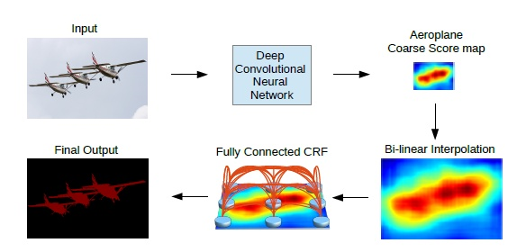

In fact, the main part of DeepLabV1 is similar to FCN, but the hole convolution is used in the last part of the sampling operation, which makes the size of the feature map keep one sixteenth. Hole convolution is a convolution technique which can increase the receptive field and keep the size of the feature image. It does not affect the effect of feature description, but also can keep rich spatial position information.

                      For example, the one-step operation of standard convolution is shown in Figure b below. The convolution kernel size is 3 × 33\times33 × 3, the step size is 2, the filling value is 1, and the receptive field size is 3 × 33\times33 × 3. The one-step operation of void / expansion convolution is shown in Figure b below. The convolution kernel size is 3 × 33\times33 × 3, the expansion rate is 2, the step size is 1, the filling value is 2, and the receptive field size is 5 × 55\times55 × 5. Although the step size is smaller, the filling is larger , but empty convolution can deal with it well and achieve the purpose mentioned above.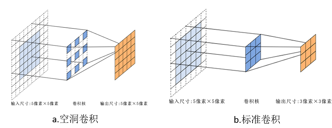

                           .

Conditional random field is a special case of Markov random field. I have drawn several diagrams to roughly describe the modeling process of fully connected conditional random field

As shown in figure a, there is a pair of original images, which should be classified pixel by pixel. Simply, the pixel category of each point is only related to itself, and figure b is obtained, which is obviously not enough. Let the pixel of each point be related to its four neighboring pixels to get figure c, but if the neighboring points fluctuate, then this degree of correlation is not enough. Let the pixels of each point be correlated with all other pixels. This correlation can be positive or negative. In this way, figure d, full connection conditional random field is obtained. It's also called Dense CRF.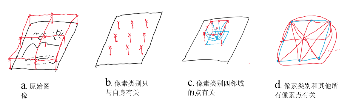

                         

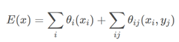
The first half of it is a univariate function, where P(xi) is a probability value generated by the deep convolution neural network: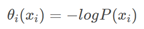

The second half of    represents the relationship between a pair of pixels, and the calculation formula is as follows: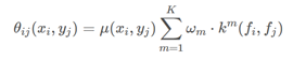

  u(xi,yj)u(x_i,y_j)u(xi, YJ) indicates the binding conduction direction, whether to enhance or weaken. For example, pixel 1 may be a person, pixel 2 may be a person, and pixel 3 may be a car, so 1 and 2 enhance each other, and 2 and 3 weaken each other. The latter weighted item is the typical score weight multiplied by the feature to calculate the intimacy between the two pixel points. The specific calculation process is as follows: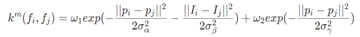

   where ppp is the 2D position of the pixel, III is the 3D pixel value of the image, with three different variance symbols representing the variance of three Gaussian distributions; the second half is a smooth processing. It can be seen from this: the closer the pixel distance is, the closer the color is, the stronger the feature will be; and if the denominator, that is, the variance is large, the feature will be difficult to be strong; so this is a process of finding similar pixels in five-dimensional space and enhancing the feature.

It seems that DenseCRF is difficult to implement, but in fact, there are packages in python that pydensecrf can implement, and as a post-processing method, it does not participate in training.

In DeepLabV1, W2, σ γ = 3w_2,\sigma_{\gamma}=3w2​,σγ​=3，w1,σalpha,σβw_1 ,\sigma_{alpha},\sigma_{\beta}w1, σ alpha, σ β are cross verified on a small data set of 100 pictures, and a rough range value is obtained, where W1 ∈ [5;10]w_1\in[5; 10]w1​∈[5;10]，σalpha∈[50:10:100]\sigma_{alpha}\in[50 : 10 : 100]σalpha​∈[50:10:100]，σβ∈[3:1:10]\sigma_{\beta}\in[3 : 1 : 10]σβ​∈[3:1:10].

3. Multiscale semantic aggregation model using void convolution

Yu F, Koltun V. Multi-Scale Context Aggregation by Dilated Convolutions[C]. international conference on learning representations, 2016.

The paper raises two questions:

• Do you really need the lower sampling layer?
• Is it necessary to analyze multiple rescaled images separately? (deep lab V1 and other models take multiple images with different resolutions as training samples)

This paper analyzes the above two problems and designs a model architecture, that is, full convolution neural network + empty convolution, front-end module + context module, as shown in the following figure: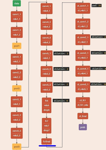

                          the front-end module is the context module before FC final, which looks like a network stack, because the front-end module is essentially an improved VGG16 (the last two pooling layers of VGG-16 are removed 4) It can complete the task of semantic segmentation independently and has a good effect.                             . The context module aims to improve the performance of semantic segmentation network structure by aggregating multi-scale context information. The. Finally, the output module is generated by executing a convolution kernel of 1 × 1 × C1\times1\times C1 × 1 × C. In particular, the basic context module is divided into two forms according to different convolution channels: basic and large. In this paper, C is 64.

4. DeepLabV2-DeepLabV1+ASPP

Chen L C , Papandreou G , Kokkinos I , et al. DeepLab: Semantic Image Segmentation with Deep Convolutional Nets, Atrous Convolution, and Fully Connected CRFs[J]. IEEE Transactions on Pattern Analysis & Machine Intelligence, 2016, 40(4):834-848.

Compared with V1, DeepLabV2 has an additional hole convolution spatial pooling feature pyramid (ASPP), which pays more attention to the problem of multi-scale targets. ASPP further utilizes void convolution, and the module structure is as follows: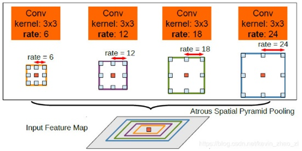

This module is used for multi-scale semantic aggregation in this paper. It discards the previous methods, such as scaling the input to multiple scales and then training, or linear aggregation of context module just mentioned. The module first performs parallel hole convolution of different sampling rates for the same input and then performs feature fusion. The hole rates used in this version of deepbab are 6, 12, 18, 24. In fact, the expansion convolution of void rate has a high demand for graphics card resources and a slow speed. Moreover, due to the emergence of ResNet, the paper uses the adjusted ResNet101 in the backbone network, which leads to the model more "heavy".

5. RefineNet multi channel fine network for high resolution image semantic segmentation

In addition to the loss of image details in the process of down sampling, two problems of void convolution are mentioned

• In essence, it is a kind of rough undersampling
• Huge computing cost

The architecture used includes:

• Rewinder neural network (ResNet)
• Multiple parallel network feature extraction
• Chain residual pooling

                            




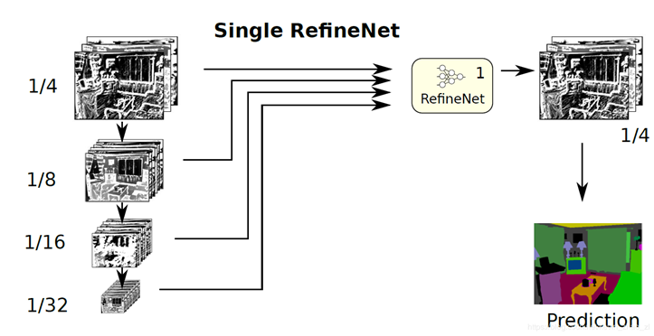
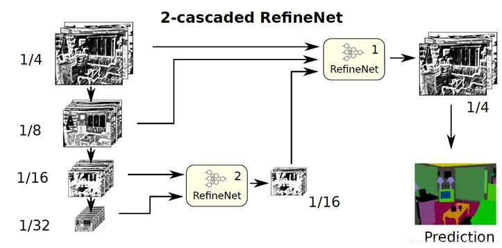
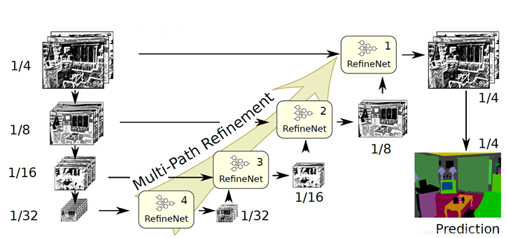
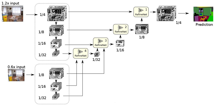
In essence, the original image has been zoomed to more scales, and this model is not easy to train. There is a RefineNet module in each of the four structures, as shown in the figure below: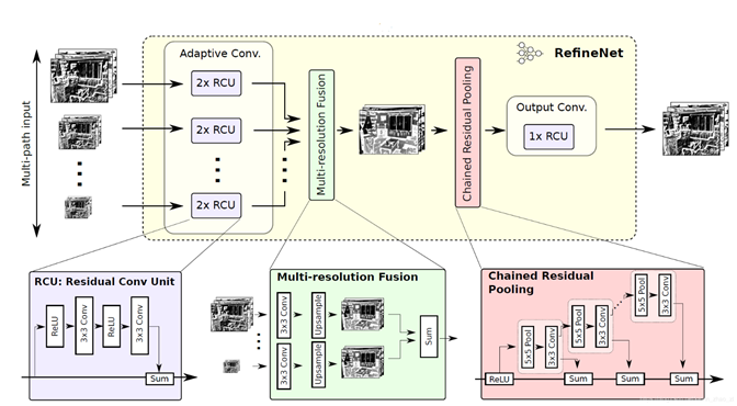

                             , RCU is a full convolution form of ResNet; multi resolution fusion is to process the same size of Solutions is mainly used to generate characteristic graphs with classification probability.

6. PSPNet - pyramid scenario analysis network

Zhao H, Shi J, Qi X, et al. Pyramid Scene Parsing Network[C]. computer vision and pattern recognition, 2017: 6230-6239.

                     

• Lack of capture of context [i.e. mutual influence of each pixel]
• Fail to make full use of the relationship between categories [e.g. ships with high probability of appearing on water, not cars]
• Weak ability to capture inconspicuous targets [small targets or similar targets block each other]
• Global average pooling results in the loss of location information [in order to obtain classification, FCN based models often directly use the global average pooling processing feature map]

Based on these problems, the paper designs the model architecture as shown in the figure below, including pyramid pooling and more effective ResNet training loss function. The model architecture is shown in the figure below: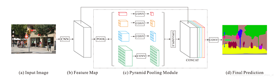

The     model uses ResNet with hole convolution as the backbone network to extract the feature map, which is 1 / 8 of the input image. After pyramidal pooling module to obtain semantic information, four different levels of pyramids are used and upper sampling is used to fuse them into the size of the original feature map. After a convolution layer, the predicted output is obtained.

                                 . Subsequent experiments show that this method is conducive to fast convergence.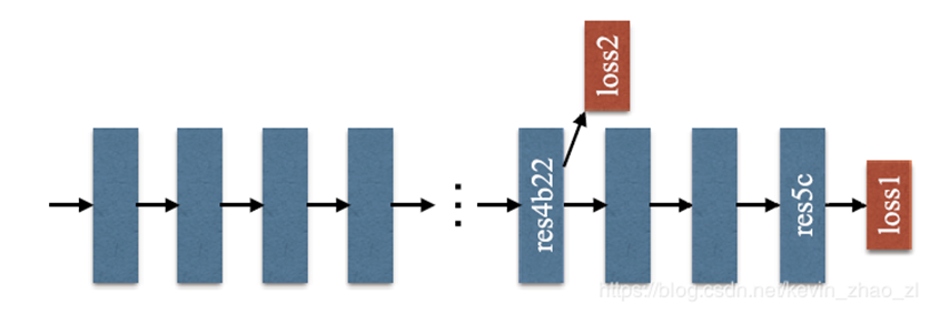

7. Deep lab V3 - Rethinking the empty convolution used in image semantic segmentation

Chen L, Papandreou G, Schroff F, et al. Rethinking Atrous Convolution for Semantic Image Segmentation[J]. arXiv: Computer Vision and Pattern Recognition, 2017.

The architecture of   model is re established as follows:

• Improved pyramid pooling of void convolution space
• Abandon all connected Airport

                             . In this paper, the tedious post-processing is abandoned, so that the model can be trained and inferred end-to-end, and some column adjustments are made in the implementation details, including learning rate strategy, batch regularization layer, backbone network pooling and hole convolution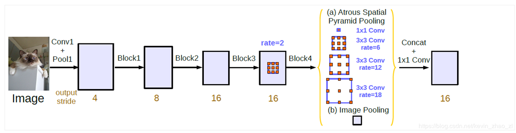

8. Deep lab V3 + encoding and decoding structure with empty convolution for image semantic segmentation

Chen L, Zhu Y, Papandreou G, et al. Encoder-Decoder with Atrous Separable Convolution for Semantic Image Segmentation[C]. european conference on computer vision, 2018: 833-851.

In this paper, DeepLabV3 is used as the encoding module to design a simple decoding module for up sampling and propose the encoding and decoding structure. The structure of this paper is shown in the following figure: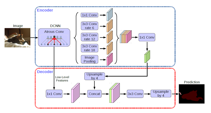

As you can see, a shallow feature is added to the decoder to increase the weight of position information.

In order to speed up the inference, the thesis improves the Xception backbone network to get a backbone network with the following characteristics:

• more layers
• All the maximum pooling operations are modified to the depth separable convolution with step size to apply the cavity separable convolution
• Additional BN and RELU activation layers are attached to each 3x3 DW Conv

The depth separable convolution is to decompose the standard convolution into a depth conv and a Pointwise Conv, where DW performs spatial convolution for each input channel independently, and PW is used to combine the output of DW. The combination of void convolution and depth separable convolution can reduce the amount of computation and keep good results.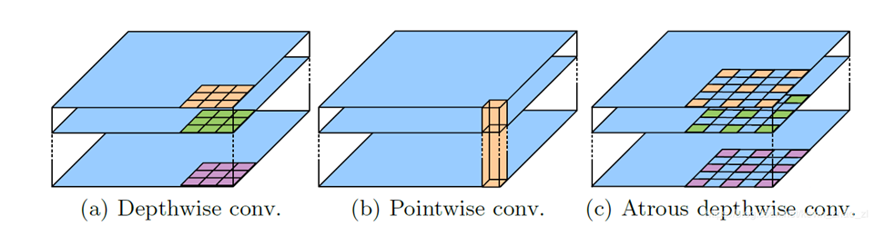

A quick look at the code:

class DeepLab(nn.Module):
    def __init__(self, backbone='resnet', output_stride=16, num_classes=21,
                 sync_bn=True, freeze_bn=False):
        super(DeepLab, self).__init__()
        if backbone == 'drn':
            output_stride = 8

        if sync_bn == True:
            BatchNorm = SynchronizedBatchNorm2d
        else:
            BatchNorm = nn.BatchNorm2d

        self.backbone = build_backbone(backbone, output_stride, BatchNorm)
        self.aspp = build_aspp(backbone, output_stride, BatchNorm)
        self.decoder = build_decoder(num_classes, backbone, BatchNorm)

        if freeze_bn:
            self.freeze_bn()

    def forward(self, input):
        x, low_level_feat = self.backbone(input)
        x = self.aspp(x)
        x = self.decoder(x, low_level_feat)
        x = F.interpolate(x, size=input.size()[2:], mode='bilinear', align_corners=True)

        return x

class Decoder(nn.Module):
    def __init__(self, num_classes, backbone, BatchNorm):
        super(Decoder, self).__init__()
        if backbone == 'resnet' or backbone == 'drn':
            low_level_inplanes = 256
        elif backbone == 'xception':
            low_level_inplanes = 128
        elif backbone == 'mobilenet':
            low_level_inplanes = 24
        else:
            raise NotImplementedError

        self.conv1 = nn.Conv2d(low_level_inplanes, 48, 1, bias=False)
        self.bn1 = BatchNorm(48)
        self.relu = nn.ReLU()
        self.last_conv = nn.Sequential(nn.Conv2d(304, 256, kernel_size=3, stride=1, padding=1, bias=False),
                                       BatchNorm(256),
                                       nn.ReLU(),
                                       nn.Dropout(0.5),
                                       nn.Conv2d(256, 256, kernel_size=3, stride=1, padding=1, bias=False),
                                       BatchNorm(256),
                                       nn.ReLU(),
                                       nn.Dropout(0.1),
                                       nn.Conv2d(256, num_classes, kernel_size=1, stride=1))
        self._init_weight()

class ASPP(nn.Module):
    def __init__(self, backbone, output_stride, BatchNorm):
        super(ASPP, self).__init__()
        if backbone == 'drn':
            inplanes = 512
        elif backbone == 'mobilenet':
            inplanes = 320
        else:
            inplanes = 2048
        if output_stride == 16:
            dilations = [1, 6, 12, 18]
        elif output_stride == 8:
            dilations = [1, 12, 24, 36]
        else:
            raise NotImplementedError

        self.aspp1 = _ASPPModule(inplanes, 256, 1, padding=0, dilation=dilations[0], BatchNorm=BatchNorm)
        self.aspp2 = _ASPPModule(inplanes, 256, 3, padding=dilations[1], dilation=dilations[1], BatchNorm=BatchNorm)
        self.aspp3 = _ASPPModule(inplanes, 256, 3, padding=dilations[2], dilation=dilations[2], BatchNorm=BatchNorm)
        self.aspp4 = _ASPPModule(inplanes, 256, 3, padding=dilations[3], dilation=dilations[3], BatchNorm=BatchNorm)

        self.global_avg_pool = nn.Sequential(nn.AdaptiveAvgPool2d((1, 1)),
                                             nn.Conv2d(inplanes, 256, 1, stride=1, bias=False),
                                             BatchNorm(256),
                                             nn.ReLU())
        self.conv1 = nn.Conv2d(1280, 256, 1, bias=False)
        self.bn1 = BatchNorm(256)
        self.relu = nn.ReLU()
        self.dropout = nn.Dropout(0.5)
        self._init_weight()

    def forward(self, x):
        x1 = self.aspp1(x)
        x2 = self.aspp2(x)
        x3 = self.aspp3(x)
        x4 = self.aspp4(x)
        x5 = self.global_avg_pool(x)
        x5 = F.interpolate(x5, size=x4.size()[2:], mode='bilinear', align_corners=True)
        x = torch.cat((x1, x2, x3, x4, x5), dim=1)

        x = self.conv1(x)
        x = self.bn1(x)
        x = self.relu(x)

        return self.dropout(x)

9. Frontier outlook in 2019

Welcome to deep learning deep in WeChat public number and mathematics, [get free daily data, AI and other related learning resources, classic and latest deep learning related papers, algorithms and other Internet skills learning, probability, linear algebra and official account of advanced mathematics knowledge).