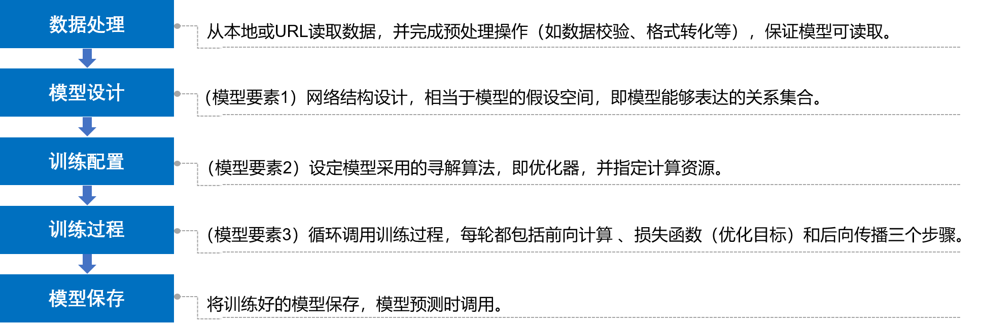
Basic steps of building deep learning model
Where to give an example: Boston house price forecast
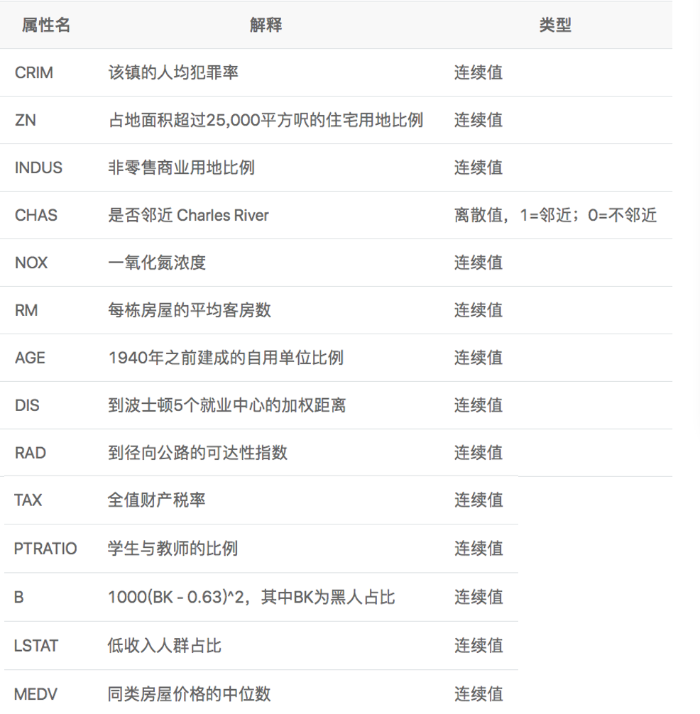
Boston house price forecasting is a classic machine learning task, similar to the "Hello World" of the programmer world. As we all know about house price, the house price in Boston area is influenced by many factors. This data set statistics 13 factors that may affect the house price and the average price of this type of house. It is expected to build a house price prediction model based on 13 factors.
1, Data processing
Data processing includes five parts: data import, data shape transformation, data set partition, data normalization and encapsulation of load data function. Data can only be called by the model after preprocessing.
1. Data shape transformation
Since the original data read in is one-dimensional, all the data are connected together. Therefore, we need to transform the shape of the data to form a two-dimensional matrix.
#Each row is a data sample, each data sample contains 13 X (characteristics affecting house price) and one Y (average price of this type of house).

feature_names = [ 'CRIM', 'ZN', 'INDUS', 'CHAS', 'NOX', 'RM', 'AGE','DIS',
                 'RAD', 'TAX', 'PTRATIO', 'B', 'LSTAT', 'MEDV' ]
feature_num = len(feature_names)
data = data.reshape([data.shape[0] // feature_num, feature_num])
'''
reshape(a,b): Become a That's ok b Column matrix
shape Read matrix length,shape[0]Is the length of the first dimension (row) of the read matrix,
'''
2. Dataset partition
The data set is divided into training set and test set, in which the training set is used to determine the parameters of the model, and the test set is used to evaluate the effect of the model.
#In this case, we use 80% of the data as a training set and 20% as a test set.
ratio = 0.8
    offset = int(data.shape[0] * ratio)
    training_data = data[:offset]
3. Data normalization
Each feature is normalized so that the value of each feature is scaled to 0 ~ 1.
There are two advantages: one is that the model training is more efficient; the other is that the weight before the feature can represent the contribution of the variable to the prediction results (because the range of each feature value itself is the same). There are two common normalization methods:
(1) Min max normalization
Also known as deviation standardization, it is a linear transformation of the original data to map the result value to [0 - 1]. The conversion function is as follows:
Where max is the maximum value of sample data and min is the minimum value of sample data. One drawback of this method is that when new data is added, it may lead to changes in max and min, which need to be redefined.
(2) Z-score standardization method
This method standardizes the mean and standard deviation of the original data. The processed data conform to the standard normal distribution, that is, the mean value is 0, the standard deviation is 1, and the conversion function is:
Where \ (\ mu \) is the mean value and \ (\ sigma \) is the standard deviation.
2, Model design
For the prediction problem, it can be divided into regression task and classification task according to whether the type of prediction output is continuous real value or discrete label. Because house price is a continuous value, house price prediction is obviously a regression task.
1. Linear regression model
It is assumed that the relationship between the house price and the influencing factors can be described in a linear way:
The solution of the model is to fit each wj and b by data. wj and b represent the weight and bias of the linear model respectively. In one-dimensional case, wj and b are the slope and intercept of the line.
The linear regression model uses the mean square error as the Loss function to measure the difference between the predicted house price and the real house price. The formula is as follows:
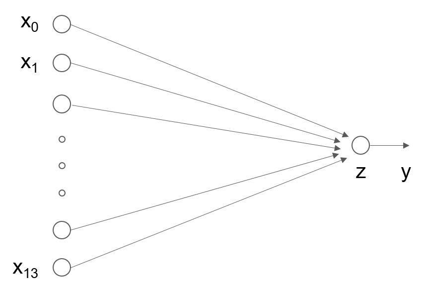
2. Neural network structure of linear regression model
In the standard structure of neural network, each neuron is composed of weighted sum and nonlinear transformation, and then multiple neurons are placed in layers and connected to form neural network. Linear regression model can be regarded as a very simple special case of neural network model. It is a neuron with only weighted sum and no nonlinear transformation (no need to form network).
3. Model design
Model design is one of the key elements of deep learning model, also known as network structure design, which is equivalent to the assumption space of the model, that is, the process of "forward calculation" (from input to output) of the model.
#If the input feature and the output predicted value are represented by vectors, the input feature x has 13 components and y has 1 component, then the shape of the parameter weight is 13 × 1.
class Network(object):
    def __init__(self, num_of_weights):
        # Initial value of randomly generated w
        # In order to maintain the consistency of the results of each run of the program,
        # Set fixed random number seed here
        np.random.seed(0)
        # NP. Random. Random() is to return one or more sample values from the standard normal distribution. The parameter is the length of each dimension of the returned matrix
        self.w = np.random.randn(num_of_weights, 1)
        self.b = 0.

     def forward(self, x):# Forward computation
        z = np.dot(x, self.w) + self.b # z = wx+b
        return z
3, Training configuration
After the completion of the model design, it is necessary to find the optimal value of the model through the training configuration, that is, to measure the quality of the model through the loss function. Training configuration is also one of the key elements of deep learning model.
For the regression problem, the most commonly used measurement method is to use the mean square error as the index to evaluate the quality of the model. The specific definition is as follows:
The Loss function in the above formula is also called Loss function, which is an indicator to measure the quality of the model. Mean square error is a common form in regression problems, and cross entropy is usually used as Loss function in classification problems.
Because the loss of each sample needs to be taken into account when calculating the loss, we need to sum the loss function of a single sample and divide it by the total number of samples N.
4, Training process
The training process is one of the key elements of the deep learning model, whose goal is to make the Loss function defined as small as possible, that is to find a parameter solution w and b to make the Loss function get the minimum value.
1. Gradient descent method
In reality, there are a lot of functions that are easy to be solved in the forward direction and difficult to be solved in the reverse direction. They are called one-way functions, so it is impossible to solve the parameter value when the derivative is 0 in the reverse direction. Then, the solution of the minimum value of Loss function can be realized by "taking the value of current parameter, descending step by step in the direction of downhill until reaching the lowest point". This method is called gradient descent method.
The scheme of gradient descent method is as follows:
- Step 1: randomly select a set of initial values, for example: [w5,w9] = [− 100.0, − 100.0]
- Step 2: select the next point [w5 ′, w9 ′], so that L(w5 ′, w9 ′) < L(w5, w9)
- Step 3: repeat step 2 until the loss function almost no longer drops.
How to choose [w5 ′, w9 ′] is very important. The first is to ensure that L is declining, and the second is to make the declining trend as fast as possible. The basic knowledge of calculus tells us that along the opposite direction of the gradient, the function value declines the fastest direction.
2. Calculation gradient
For the above calculation method of loss function, we slightly rewrite the function and introduce factor 1 / 2 (because partial derivative is needed in gradient calculation, 1 / 2 can be eliminated and calculation can be simplified). The definition of loss function is as follows:
Where zi is the prediction value of the network for the ith sample:
Gradient is defined as:
Then the partial derivatives of L to w and b are:
Here we consider the gradient calculation with only one sample:
You can calculate:
Then the partial derivatives of L to w and b are:
# According to the above formula, when there is only one sample, the gradient of a certain wj, such as w0, can be calculated.
gradient_w0 = (z1 - y1) * x1[0]
# w1
gradient_w1 = (z1 - y1) * x1[1]
# w2
gradient_w2 = (z1 - y1) * x1[2]
...

#So we can calculate all the weight gradients from w0 to w12 through for loop, or we can use numpy
Based on the Numpy broadcast mechanism (the calculation of vector and matrix is the same as that of a single variable), the gradient calculation can be realized more quickly.
#In the code of gradient calculation, we directly use (z1 - y1) * x1 to get a 13 dimensional vector, and each component represents the gradient of the dimension.
gradient_w = (z1 - y1) * x1

#Similarly, we can calculate the contribution of each sample (xi, yi) to the gradient in the form of a for loop, or we can still use numpy

# Note that this is the data of three samples at a time, not the third sample
x3samples = x[0:3]
y3samples = y[0:3]
z3samples = np.dot(x3samples, w) + b # np.dot() is matrix multiplication
gradient_w = (z3samples - y3samples) * x3samples #Contribution of the first three samples to the gradient

# So we can directly calculate the contribution of all samples to the gradient at one time
z = np.dot(x, w) + b
gradient_w = (z - y) * x #Contribution of the first three samples to the gradient
For the case of N samples, we can directly use the following method to calculate the contribution of all samples to the gradient, which is the convenience of using the Numpy library broadcast function. The advantages are:
- On the one hand, the dimension of parameters can be extended to calculate the gradient of all parameters from w0 to w12 for one sample instead of for loop.
- On the other hand, we can extend the dimension of samples, instead of for loop, to calculate the gradient of sample 0 to sample 403.
According to the formula of gradient, the total gradient is the average contribution of each sample to the gradient.
We can also use Numpy's mean function to do this:
# axis = 0 means add each row and divide by the total number of rows
gradient_w = np.mean(gradient_w, axis=0) # Get a 1-dimensional 13 column variable
We use numpy's matrix operation to easily complete the calculation of gradient, but introduce a problem: the shape of gradient_w is (13,), and the dimension of W is (13, 1). The reason for this problem is that dimension 0 is eliminated when using the np.mean function. In order to calculate conveniently, such as addition, subtraction, multiplication and division, the shape of gradient and W must be consistent. Therefore, we also set the dimension of grade_wto (13, 1)
gradient_w = gradient_w[:, np.newaxis]
The complete code for calculating the gradient is:
z = np.dot(x, w) + b
gradient_w = (z - y) * x
gradient_w = np.mean(gradient_w, axis=0)
gradient_w = gradient_w[:, np.newaxis]
For b, we also calculate the gradient in the same way
gradient_b = (z - y)
gradient_b = np.mean(gradient_b)
# Here b is a number, so you can directly use np.mean to get a scalar
gradient_b
3. Identify points with smaller loss functions
How to update the parameters to find the smaller points of Loss? It is easy to think that a small step in the opposite direction of the gradient will reduce the Loss function at the next point.
# eta: to control the change of each parameter value along the opposite direction of the gradient, that is, the step length of each movement, also known as learning rate.
eta = 0.1
# Update parameters w5 and w9
w = w - eta * gradient_w # Take a step in the opposite direction of the gradient
The sample code of Boston house price forecast from data processing to now is as follows:
import numpy as np
import json
import os
import matplotlib.pyplot as plt
from mpl_toolkits.mplot3d import Axes3D

def load_data():# data processing
    # Import data from file
    datafile = 'F:\ZTR\Study\Code\Python\.vscode\Boston\data\housing.data'
    data = np.fromfile(datafile, sep=' ')
    # The read in data is converted into 1-D array
    feature_names = [ 'CRIM', 'ZN', 'INDUS', 'CHAS', 'NOX', 'RM', 'AGE', \
                      'DIS', 'RAD', 'TAX', 'PTRATIO', 'B', 'LSTAT', 'MEDV' ]
    feature_num = len(feature_names)
    # Reshape the original data to a shape like [N, 14]
    data = data.reshape([data.shape[0] // feature_num, feature_num])

    # Split the original data set into training set and test set
    ratio = 0.8
    offset = int(data.shape[0] * ratio)
    training_data = data[:offset]

	#Calculate the maximum, minimum and average values
    maximums = training_data.max(axis=0)
    minimums = training_data.min(axis=0)
    avgs = training_data.sum(axis=0) / training_data.shape[0]

    # Normalize the data
    for i in range(feature_num):
        #print(maximums[i], minimums[i], avgs[i])
        data[:, i] = (data[:, i] - avgs[i]) / (maximums[i] - minimums[i])

    # Partition ratio of training set and test set
    training_data = data[:offset]
    test_data = data[offset:]
    return training_data, test_data

class Network(object):
    def __init__(self, num_of_weights):
        # Initial value of randomly generated w
        # In order to maintain the consistency of the results of each run of the program, a fixed random number seed is set here
        np.random.seed(0)
        self.w = np.random.randn(num_of_weights, 1)
        self.b = 0.

    def forward(self, x):# Forward calculation
        z = np.dot(x, self.w) + self.b
        return z

    def loss(self, z, y):# loss function
        error = z - y
        num_samples = error.shape[0]
        cost = error * error
        cost = np.sum(cost) / num_samples
        return cost

    def gradient(self, x, y):# Gradient computation
        z = self.forward(x)
        gradient_w = (z-y)*x
        gradient_w = np.mean(gradient_w, axis=0)
        gradient_w = gradient_w[:, np.newaxis]
        gradient_b = (z - y)
        gradient_b = np.mean(gradient_b)
        return gradient_w, gradient_b

    def update(self, gradient_w, gradient_b, eta = 0.01):# Update parameters
        self.w = self.w - eta * gradient_w
        self.b = self.b - eta * gradient_b

    def train(self, x, y, iterations=100, eta=0.01):# Training process
        losses = []
        for i in range(iterations):
            z = self.forward(x)
            L = self.loss(z, y)
            gradient_w, gradient_b = self.gradient(x, y)
            self.update(gradient_w, gradient_b, eta)
            losses.append(L)
            if (i+1) % 10 == 0:
                print('iter {}, loss {}'.format(i, L))
        return losses

# get data
train_data, test_data = load_data()
x = train_data[:, :-1]
y = train_data[:, -1:]
# Create network
net = Network(13)
num_iterations=1000
# Start up training
losses = net.train(x,y, iterations=num_iterations, eta=0.01)

# Draw the trend of loss function
plot_x = np.arange(num_iterations)
plot_y = np.array(losses)
plt.plot(plot_x, plot_y)
plt.show()
4. Random gradient descent method
In the above method, each loss function and gradient calculation is based on the total data in the data set. It is suitable for tasks with a small number of samples. However, in practical problems, data sets are often very large. If full data is used for calculation every time, the efficiency is very low. Since the parameters only update a little bit in the opposite direction of the gradient at a time, the direction does not need to be so precise. A reasonable solution is to randomly extract a small part of data from the total data set each time to represent the whole. Based on this part of data, calculate the gradient and loss to update the parameters. This method is called the Stochastic Gradient Descent (SGD). The core concepts are as follows:
- Min batch: a batch of data extracted at each iteration is called a min batch.
- Batch size: the number of samples contained in a mini batch is called batch size.
- Epoch: when the program iterates, the samples are gradually extracted according to mini batch. When the entire data set is traversed, a round of training, also called an epoch, is completed. When starting a training, you can pass in the number of rounds of training, Num? Epichs and batch? Size, as parameters.
- iterations: the number of batch es required to complete an epoch.
The following describes the specific implementation process with the program, involving data processing and training process two parts of the code modification.
(1) Code modification of data processing part
Data processing needs two functions: splitting data batches and disordering samples (in order to achieve the effect of random sampling).
# get data
train_data, test_data = load_data()

# There are 404 pieces of data in train data. If batch size = 10, take the first 0-9 sample as the first mini batch, and name train data 1.
train_data1 = train_data[0:10]
# Use the data (sample no.0-9) of the train? Data1 to calculate the gradient and update the network parameters.
net = Network(13)
x = train_data1[:, :-1]
y = train_data1[:, -1:]
loss = net.train(x, y, iterations=1, eta=0.01)
# According to this method, new mini batch is taken out and network parameters are updated gradually. (samples 10-19, 20-29...)
Next, divide the train data into multiple mini batch with the size of batch.
# The train data is divided into 404 / 10 + 1 Mini batch, of which the first 40 Mini batch contain 10 samples, and the last Mini batch contain only 4 samples.
batch_size = 10
n = len(train_data)
mini_batches = [train_data[k:k+batch_size] for k in range(0, n, batch_size)]
Through a large number of experiments, it is found that the model is more impressed by the final data. After the training data is imported, the closer to the end of the model training, the greater the impact of the last batch data on the model parameters. In order to avoid the influence of model memory on training effect, it is necessary to carry out the operation of sample disorder.
'''
//Here we take out mini_batch in order, while in SGD (random gradient descent), we take a part of samples randomly to represent the population. In order to achieve the effect of random sampling, we first randomly scramble the sample order in the train data, and then extract mini_batch.
'''
np.random.shuffle(train_data)
======================================
# The final code of data processing part is as follows:
# get data
train_data, test_data = load_data()
# Scramble sample order
np.random.shuffle(train_data)
# Divide train data into multiple mini batch
batch_size = 10
n = len(train_data)
mini_batches = [train_data[k:k+batch_size] for k in range(0, n, batch_size)]
# Create network
net = Network(13)
# Use the data of each mini batch in turn
for mini_batch in mini_batches:
    x = mini_batch[:, :-1]
    y = mini_batch[:, -1:]
    loss = net.train(x, y, iterations=1)
(2) Training process code modification
Each randomly selected Mini batch data is input into the model for parameter training. The core of the training process is two levels of circulation:
i. The first level loop, which represents the sample set to be trained to traverse several times, is called "epoch".
for epoch_id in range(num_epoches):
ii. The second level loop, which represents the multiple batches that the sample set is split into each time it is traversed, requires all the training, which is called "iter (iteration).". for iter_id,mini_batch in emumerate(mini_batches):
Inside the two-level loop is the classic four-step training process: forward calculation - > calculation loss - > calculation gradient - > update parameters
5, Final full code
import numpy as np
import json
import os
import matplotlib.pyplot as plt
from mpl_toolkits.mplot3d import Axes3D

#================Data processing==================
def load_data():
    # Import data from file
    datafile = 'F:\ZTR\Study\Code\Python\.vscode\Boston\data\housing.data'
    data = np.fromfile(datafile, sep=' ')

    # After reading in, the data is converted into 1-D array, in which 0-13 items of array are the first data, 14-27 items are the second data, and so on
    # Each data includes 14 items, of which the first 13 items are the influencing factors, and the 14th item is the corresponding median housing price
    feature_names = [ 'CRIM', 'ZN', 'INDUS', 'CHAS', 'NOX', 'RM', 'AGE', \
                      'DIS', 'RAD', 'TAX', 'PTRATIO', 'B', 'LSTAT', 'MEDV' ]
    feature_num = len(feature_names)
    # Reshape the original data to a shape like [N, 14]
    data = data.reshape([data.shape[0] // Shape (row, column) is used to read the length of the matrix, and shape[0] is the length of the first dimension of the read matrix

    # Split the original data set into training set and test set
    # 80% of the data is used for training and 20% for testing
    # There must be no intersection between test set and training set
    ratio = 0.8
    offset = int(data.shape[0] * ratio)
    training_data = data[:offset]

     #Data normalization
    '''
    //Each feature is normalized so that the value of each feature is scaled to 0 ~ 1. There are two benefits to doing so:
    //First, model training is more efficient;
    //Second, the weight before the feature can represent the contribution of the variable to the prediction results (because the range of each feature value itself is the same).
    '''
    # Calculate the maximum, minimum and average value of the train data set
    maximums = training_data.max(axis=0) #Axis is the matrix dimension, for example, axis=0 is the first dimension, that is, row; axis=1 is the second dimension, that is, column
    minimums = training_data.min(axis=0)
    avgs = training_data.sum(axis=0) / training_data.shape[0]

    # Normalize the data
    for i in range(feature_num):
        #print(maximums[i], minimums[i], avgs[i])
        data[:, i] = (data[:, i] - avgs[i]) / (maximums[i] - minimums[i])#The calculation method is in doubt. data[:,i] refers to the ith element of each line

    # Partition ratio of training set and test set
    training_data = data[:offset]
    test_data = data[offset:]
    return training_data, test_data

#================Model design==================
'''
//Model design is one of the key elements of deep learning model, also known as network structure design, which is equivalent to the assumption space of the model, that is, the process of "forward calculation" (from input to output) of the model.
//If the input feature and the output predicted value are represented by vectors, the input feature x has 13 components and y has 1 component, then the shape of the parameter weight is 13 × 1.
'''

'''
//The above process of calculating the predicted output is described in the way of "class and object". The class member variables include the parameters w and b.
//By writing a forward function (for forward calculation), the calculation process from features and parameters to output predicted value is completed.
'''
class Network(object):
    def __init__(self, num_of_weights):
        # Initial value of randomly generated w
        # In order to maintain the consistency of the results of each run of the program,
        # Set fixed random number seed here
        np.random.seed(0)
        self.w = np.random.randn(num_of_weights, 1)# NP. Random. Random() is to return one or more sample values from the standard normal distribution. The parameter is the length of each dimension of the returned matrix
        self.b = 0.

    def forward(self, x):
        z = np.dot(x, self.w) + self.b
        return z

    # Training configuration
    # After the completion of the model design, we need to find the optimal value of the model through the training configuration, that is, to measure the quality of the model through the loss function. Training configuration is also one of the key elements of deep learning model.
    '''
    //For the regression problem, the most commonly used measurement method is to use the mean square error as the index to evaluate the quality of the model. The specific definition is as follows:
    Loss=(y−z)^2
    //The Loss function in the above formula is also called Loss function, which is an indicator to measure the quality of the model.
    //In the regression problem, the mean square error is a common form. In the classification problem, the cross entropy is usually used as the loss function,
    '''
    def loss(self, z, y):
        error = z - y
        num_samples = error.shape[0]
        cost = error * error
        cost = np.sum(cost) / num_samples
        return cost

    # Training process
    '''
    //The steps of gradient descent method are as follows:
    //Step 1: randomly select a set of initial values, for example: [w 5, w9] = [− 100.0, − 100.0] [w5,w9] = [- 100.0, - 100.0]
    //Step 2: select the next point [w5 ′, w9 ′], so that L(w5 ′, w9 ′) < L(w5, w9)
    //Step 3: repeat step 2 until the loss function almost no longer drops.
    '''
    def gradient(self, x, y):
        z = self.forward(x)
        gradient_w = (z-y)*x
        gradient_w = np.mean(gradient_w, axis=0)
        gradient_w = gradient_w[:, np.newaxis]
        gradient_b = (z - y)
        gradient_b = np.mean(gradient_b)
        return gradient_w, gradient_b

    def update(self, gradient_w, gradient_b, eta = 0.01):
        self.w = self.w - eta * gradient_w
        self.b = self.b - eta * gradient_b

    def train(self, training_data, num_epoches, batch_size=10, eta=0.01):
        n = len(training_data)
        losses = []
        for epoch_id in range(num_epoches):
            # Before each iteration, the order of training data is randomly disrupted,
            np.random.shuffle(training_data)
            # Then take out the data in the way of taking batch ﹣ size bar every time
            # Split the training data. Each mini batch contains the data of the batch size bar
            mini_batches = [training_data[k:k+batch_size] for k in range(0, n, batch_size)]

            for iter_id, mini_batch in enumerate(mini_batches):# The purpose of enumerate() is to combine a traversable data object into an index sequence and list data and data subscripts at the same time
                #print(self.w.shape)
                #print(self.b)
                x = mini_batch[:, :-1]
                y = mini_batch[:, -1:]
                a = self.forward(x)
                loss = self.loss(a, y)
                gradient_w, gradient_b = self.gradient(x, y)
                self.update(gradient_w, gradient_b, eta)
                losses.append(loss)
                print('Epoch {:3d} / iter {:3d}, loss = {:.4f}'.
                                 format(epoch_id, iter_id, loss))

        return losses

# get data
train_data, test_data = load_data()
# Scramble sample order
np.random.shuffle(train_data)
# Divide train data into multiple mini batch
batch_size = 10
n = len(train_data)
mini_batches = [train_data[k:k+batch_size] for k in range(0, n, batch_size)]
# Create network
net = Network(13)

# Start up training
losses = net.train(train_data, num_epoches=50, batch_size=100, eta=0.1)

# Draw the trend of loss function
plot_x = np.arange(len(losses))
plot_y = np.array(losses)
plt.plot(plot_x, plot_y)
plt.show()

'''
//There are three main points to use neural network to model house price forecast:
1,Build network, initialize parameters w and b,Define the calculation method of prediction and loss function.
2,The initial point is selected randomly, and the gradient calculation method and parameter updating method are established.
3,Extract part of the data from the total data set as a mini_batch,The gradient is calculated and the parameters are updated, and iteration is continued until the loss function almost no longer drops.
'''