Author: xiaoyu
WeChat official account: Python Data Science
Purpose: This article introduces you to a primary project of data analysis. The purpose is to understand how to use Python for simple data analysis through the project.
Data source: Bloggers collect official account data of Beijing secondary housing through crawler collection (full back of the public network).
Preliminary study on data
First, import the scientific computing packages numpy,pandas, visual matplotlib,seaborn, and machine learning package sklearn.
import pandas as pd
import numpy as np
import seaborn as sns
import matplotlib as mpl

import matplotlib.pyplot as plt
from IPython.display import display
plt.style.use("fivethirtyeight")
sns.set_style({'font.sans-serif':['simhei','Arial']})
%matplotlib inline


# Check Python version
from sys import version_info
if version_info.major != 3:
    raise Exception('Please use Python 3 To complete this project')
Copy code
Then import the data and make preliminary observations. These observations include understanding the missing values, outliers and approximate descriptive statistics of data characteristics.
# Import chain home second-hand housing data
lianjia_df = pd.read_csv('lianjia.csv')
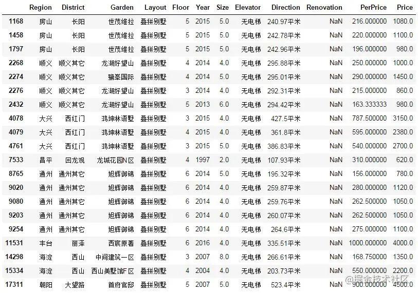
display(lianjia_df.head(n=2))
Copy code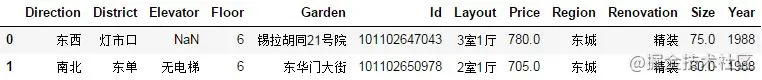
It is preliminarily observed that there are 11 characteristic variables. Price is our target variable here, and then we continue to observe it in depth.
# Check for missing values
lianjia_df.info()
Copy code
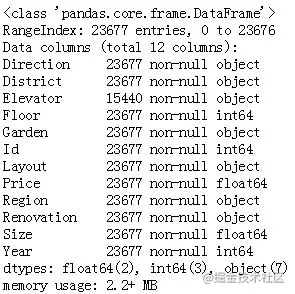
It is found that there are 23677 pieces of data in the data set, of which the Elevator feature has obvious missing values.
lianjia_df.describe()
Copy code
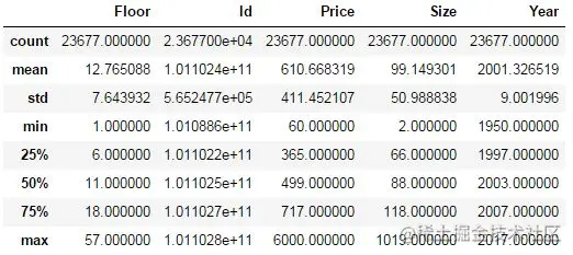
The above results give some statistical values of eigenvalues, including mean, standard deviation, median, minimum, maximum, 25% quantile and 75% quantile. These statistical results are simple and direct, which is very useful for the initial understanding of the quality of a feature. For example, we observed that the maximum value of the Size feature is 1019 square meters and the minimum value is 2 square meters. Then we need to think about whether this exists in practice. If it does not exist, it is meaningless, then this data is an abnormal value, which will seriously affect the performance of the model.
Of course, this is only a preliminary observation. Later, we will use data visualization to clearly show and confirm our guess.
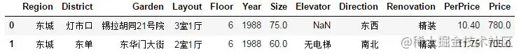
# Add new features and average house price
df = lianjia_df.copy()
df['PerPrice'] = lianjia_df['Price']/lianjia_df['Size']

# Reposition columns
columns = ['Region', 'District', 'Garden', 'Layout', 'Floor', 'Year', 'Size', 'Elevator', 'Direction', 'Renovation', 'PerPrice', 'Price']
df = pd.DataFrame(df, columns = columns)

# Revisit the dataset
display(df.head(n=2))
Copy code
We found that the Id feature has no practical significance, so we removed it. Since the house unit price is easy to analyze and can be obtained simply by using the total price / area, a new feature PerPrice (only for analysis, not for prediction) is added. In addition, the order of features has been adjusted to look more comfortable.
Data visualization analysis
Region feature analysis
For regional characteristics, we can analyze the comparison of house prices and quantities in different regions.
# Compare the number of second-hand houses and the house price per square meter by regional grouping of second-hand houses
df_house_count = df.groupby('Region')['Price'].count().sort_values(ascending=False).to_frame().reset_index()
df_house_mean = df.groupby('Region')['PerPrice'].mean().sort_values(ascending=False).to_frame().reset_index()

f, [ax1,ax2,ax3] = plt.subplots(3,1,figsize=(20,15))
sns.barplot(x='Region', y='PerPrice', palette="Blues_d", data=df_house_mean, ax=ax1)
ax1.set_title('Comparison of unit price per square meter of second-hand houses in Beijing',fontsize=15)
ax1.set_xlabel('region')
ax1.set_ylabel('Unit price per square meter')

sns.barplot(x='Region', y='Price', palette="Greens_d", data=df_house_count, ax=ax2)
ax2.set_title('Comparison of the number of second-hand houses in Beijing',fontsize=15)
ax2.set_xlabel('region')
ax2.set_ylabel('quantity')

sns.boxplot(x='Region', y='Price', data=df, ax=ax3)
ax3.set_title('Total price of second-hand houses in Beijing',fontsize=15)
ax3.set_xlabel('region')
ax3.set_ylabel('Total house price')

plt.show()
Copy code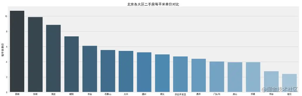
The network perspective function of pandas is used to sort groups by groups. The visualization of regional features is directly completed by seaborn. The palette palette parameter is used for color. The lighter the color gradient, the less the description, and vice versa. It can be observed that:
- Average price of second-hand houses: the house price in Xicheng District is the most expensive, and the average price is about 110000 / Ping, because Xicheng is within the second ring road and is the gathering place of popular school district houses. The second is about 100000 / ping in Dongcheng, then about 85000 / ping in Haidian, and the others are lower than 80000 / Ping.
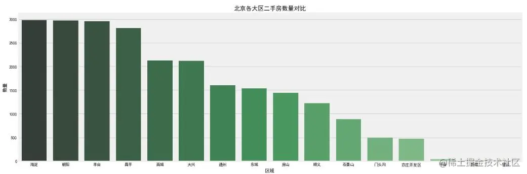
- Number of second-hand houses: statistically speaking, there are hot areas in the second-hand house market. Haidian District and Chaoyang District have the largest number of second-hand houses, almost close to 3000 sets. After all, there is a large demand in the region. Then there is Fengtai District, which is under transformation and construction in recent years and has the potential to catch up with and surpass.
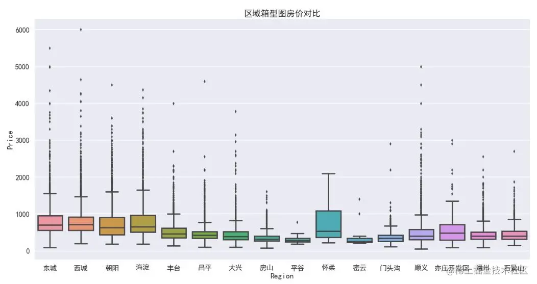
- Total price of second-hand houses: according to the box chart, the median total price of houses in all major regions is less than 10 million, and the discrete value of total price of houses is high, with the highest value of 60 million in Xicheng, indicating that the characteristics of house price are not ideal Zhengtai distribution.
Size feature analysis
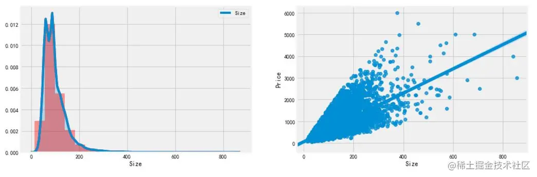
f, [ax1,ax2] = plt.subplots(1, 2, figsize=(15, 5))
# Distribution of building time
sns.distplot(df['Size'], bins=20, ax=ax1, color='r')
sns.kdeplot(df['Size'], shade=True, ax=ax1)
# Relationship between building time and selling price
sns.regplot(x='Size', y='Price', data=df, ax=ax2)
plt.show()
Copy code
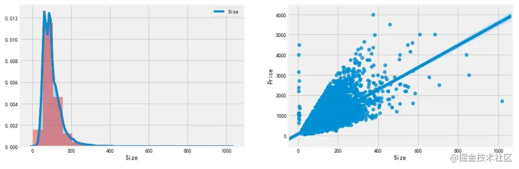
- Size distribution: use distplot and kdeplot to draw a histogram to observe the distribution of size characteristics, which belongs to the distribution of long tail type, which shows that there are many second-hand houses with large area and beyond the normal range.
- Relationship between Size and Price: the scatter diagram between Size and Price is drawn through regplot. It is found that the Size feature basically has a linear relationship with Price, which is in line with basic common sense. The larger the area, the higher the Price. However, there are two groups of obvious anomalies: 1. The area is less than 10 square meters, but the Price exceeds 100 million; 2. The area of a point exceeds 1000 square meters and the Price is very low. You need to check the situation.
df.loc[df['Size']< 10]
Copy code
After checking, it is found that this group of data is a villa. The reason for the abnormality is that the villa structure is special (no orientation and no elevator), and the field definition is different from that of second-hand commercial housing, resulting in the dislocation of crawler crawling data. Because the second-hand house of villa type is not within our consideration, it is removed and the relationship between Size distribution and Price is observed again.
df.loc[df['Size']>1000]
Copy code

After observation, this abnormal point is not an ordinary civil second-hand house, but probably a commercial house. Therefore, there is 1 room and 0 hall with such a large area of more than 1000 square meters, so we choose to remove it here.
df = df[(df['Layout']!='stacked townhouse')&(df['Size']<1000)]
Copy code
No obvious outliers are found after re visualization.
Layout feature analysis
f, ax1= plt.subplots(figsize=(20,20))
sns.countplot(y='Layout', data=df, ax=ax1)
ax1.set_title('House type',fontsize=15)
ax1.set_xlabel('quantity')
ax1.set_ylabel('House type')
plt.show()
Copy code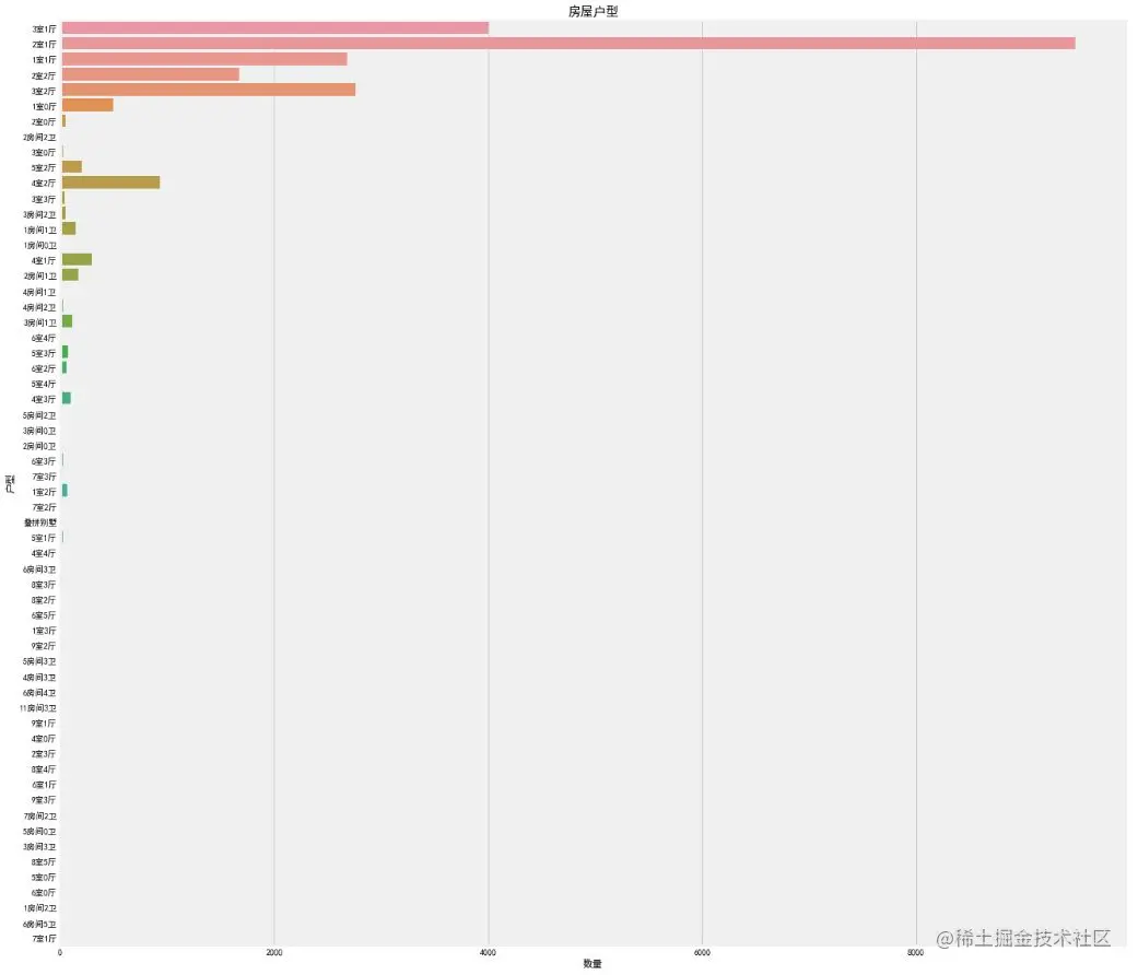
This feature is really unknown. There are strange structures such as 9 rooms, 3 rooms, 4 rooms and 0 rooms. Among them, two bedrooms and one living room account for the vast majority, followed by three bedrooms and one living room, two bedrooms and two living rooms. However, after careful observation, there are many irregular names under the feature classification, such as 2 bedrooms and 1 living room, 2 bedrooms and 1 bathroom, and villas. There is no unified name. Such features can not be used as the data input of machine learning model, and feature engineering needs to be used for corresponding processing.
Innovation feature analysis
df['Renovation'].value_counts()
Copy code
Hardcover 11345
Paperback 8497
Others 3239
Blank 576
North south 20
Name: Renovation, dtype: int64
It is found that there are north and South in the Renovation decoration features, which belongs to the orientation type. It may be that some information positions are empty during the reptile process, resulting in the "Direction" orientation feature appearing here, so it needs to be removed or replaced.
# Remove the error data "north and South", because some information positions are empty during the crawling process, resulting in the presence of the "Direction" feature, which needs to be cleared or replaced
df['Renovation'] = df.loc[(df['Renovation'] != 'north and south'), 'Renovation']

# Frame setting
f, [ax1,ax2,ax3] = plt.subplots(1, 3, figsize=(20, 5))
sns.countplot(df['Renovation'], ax=ax1)
sns.barplot(x='Renovation', y='Price', data=df, ax=ax2)
sns.boxplot(x='Renovation', y='Price', data=df, ax=ax3)
plt.show()
Copy code
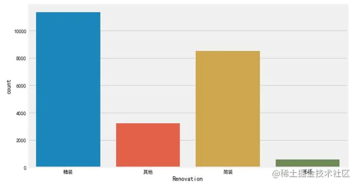
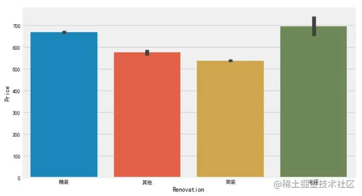
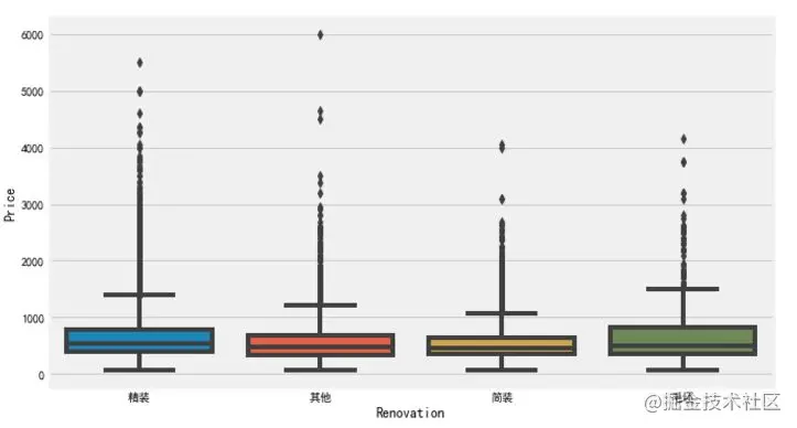
It is observed that the number of second-hand houses with fine decoration is the largest, followed by simple decoration, which is also common in our weekdays. For the price, the blank type is the highest, followed by fine decoration.
Elevator feature analysis
When exploring the data, we found that the Elevator feature has a large number of missing values, which is very unfavorable to us. First, let's see how many missing values there are:
misn = len(df.loc[(df['Elevator'].isnull()), 'Elevator'])
print('Elevator The number of missing values is:'+ str(misn))
Copy code
Number of missing values for Elevator: 8237
What about so many missing values? This needs to be considered according to the actual situation. The commonly used methods include average / median filling method, direct removal, or modeling and prediction according to other features.
Here we consider the filling method, but whether there is an elevator is not a numerical value, and there is no mean and median. How to fill it? Here is an idea for you: judge whether there is an elevator according to the Floor. Generally, there are elevators on floors greater than 6, while there are generally no elevators on floors less than or equal to 6. With this standard, the rest is simple.
# Due to individual types of errors, such as simple and hardcover, the eigenvalues are misaligned, so they need to be removed
df['Elevator'] = df.loc[(df['Elevator'] == 'There is an elevator')|(df['Elevator'] == 'No elevator'), 'Elevator']

# Fill in the missing value of Elevator
df.loc[(df['Floor']>6)&(df['Elevator'].isnull()), 'Elevator'] = 'There is an elevator'
df.loc[(df['Floor']<=6)&(df['Elevator'].isnull()), 'Elevator'] = 'No elevator'

f, [ax1,ax2] = plt.subplots(1, 2, figsize=(20, 10))
sns.countplot(df['Elevator'], ax=ax1)
ax1.set_title('Comparison of elevator quantity',fontsize=15)
ax1.set_xlabel('Is there an elevator')
ax1.set_ylabel('quantity')
sns.barplot(x='Elevator', y='Price', data=df, ax=ax2)
ax2.set_title('Comparison of house price with and without elevator',fontsize=15)
ax2.set_xlabel('Is there an elevator')
ax2.set_ylabel('Total price')
plt.show()
Copy code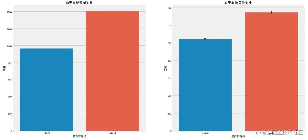
It is observed that the number of second-hand houses with elevators is in the majority. After all, the high-rise land utilization rate is relatively high, which is suitable for the needs of the huge population in Beijing, and the high-rise buildings need elevators. Accordingly, the house price of second-hand houses with elevators is higher, because the early decoration fee and later maintenance fee of elevators are included (but this price comparison is only an average concept. For example, the price of a 6-storey luxury community without elevators is certainly higher).
Year feature analysis
grid = sns.FacetGrid(df, row='Elevator', col='Renovation', palette='seismic',size=4)
grid.map(plt.scatter, 'Year', 'Price')
grid.add_legend()
Copy code
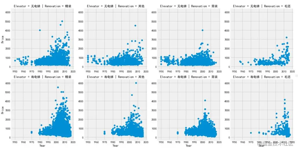
Under the classification conditions of Renovation and Elevator, the Year features are analyzed by FaceGrid. The observation results are as follows:
- The whole second-hand housing price trend increases with time;
- The house prices of second-hand houses built after 2000 have increased significantly compared with those before 2000;
- Before 1980, there was almost no data on second-hand houses with elevators, indicating that there was no large-scale installation of elevators before 1980;
- Before 1980, among the second-hand houses without elevators, the simple decoration second-hand houses accounted for the vast majority, while the hard decoration was very few;
Floor feature analysis
f, ax1= plt.subplots(figsize=(20,5))
sns.countplot(x='Floor', data=df, ax=ax1)
ax1.set_title('House type',fontsize=15)
ax1.set_xlabel('quantity')
ax1.set_ylabel('House type')
plt.show()
Copy code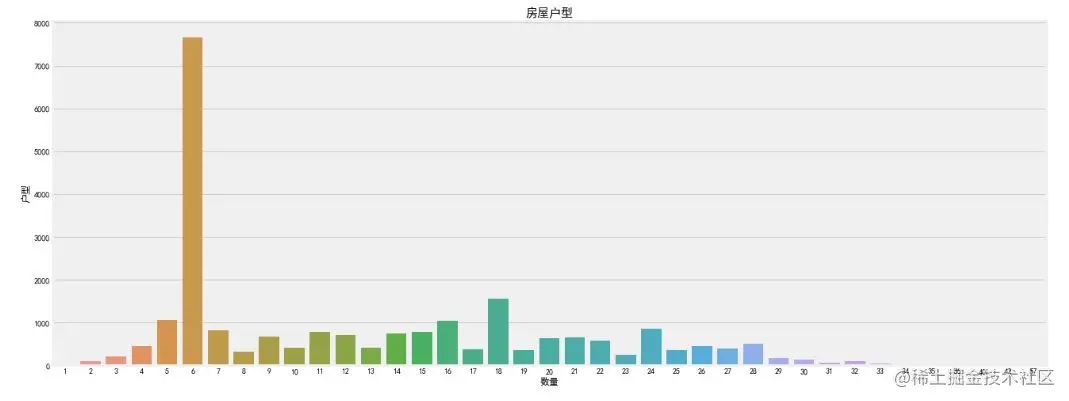
It can be seen that the number of second-hand houses with six floors is the largest, but the individual floor characteristics are meaningless, because the total number of floors of houses in each community is different. We need to know the relative significance of floors. In addition, there is also a very important connection between the floor and culture. For example, Chinese culture is seven up and eight down. The seventh floor may be popular and the house price is expensive. Generally, there will not be four floors or 18 floors. Of course, under normal circumstances, the middle floor is more popular and the price is high. The popularity of the ground floor and the top floor is low and the price is relatively low. Therefore, the floor is a very complex feature, which has a great impact on the house price.
summary
This sharing aims to let you know how to do a simple data analysis with Python. It is undoubtedly a good exercise for friends who have just come into contact with data analysis. However, there are still many problems to be solved in this analysis, such as:
- Solve the problem of data source accuracy obtained by crawler;
- Need to crawl or find more good selling features;
- More feature engineering work needs to be done, such as data cleaning, feature selection and screening;
- Use statistical model to establish regression model for price prediction;
More content will be introduced and shared slowly. Please look forward to it.
Author: Python Data Science
Link: https://juejin.cn/post/6844903630437384200