The basic operations of Python numpy are not common to you

Keywords: Python MATLAB Attribute

The text and pictures of this article are from the Internet, only for learning and communication, not for any commercial purpose. The copyright belongs to the original author. If you have any questions, please contact us in time for handling.
PS: if you need the latest Python learning materials, you can click the link below to get them by yourself
http://note.youdao.com/noteshare?id=a3a533247e4c084a72c9ae88c271e3d1

Look at the text:

0, NumPy and Darry

NumPy is the basic package of Python scientific computing, which is produced for strict digital processing.

It provides:

Fast and efficient multidimensional array object ndarray;
Functions that directly perform mathematical operations on arrays and element level calculations on arrays;
Linear algebra operation and random number generation;
Integrate C, C + +, Fortran code into Python tools, etc.

It is designed for rigorous digital processing. Most of them are used by many large financial companies, as well as core scientific computing organizations, such as Lawrence Livermore and NASA, which are used to deal with some tasks originally done using C + +, Fortran or Matlab.

ndarray is a multi-dimensional array object, which has the ability of vector arithmetic operation and complex broadcast, and has the characteristics of fast execution and space saving.

One of the characteristics of ndarray is Isomorphism: all elements must be of the same type.

1. View array properties: type, size, shape, dimension

import numpy as np  
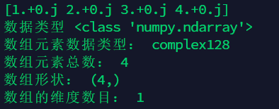
a1 = np.array([1,2,3,4],dtype=np.complex128)  
print(a1)  
print("data type",type(a1))           #Print array data type  
print("Array element data type:",a1.dtype) #Print array element data type  
print("Total array elements:",a1.size)      #Print array size, that is, the total number of array elements  
print("Array shape:",a1.shape)         #Print array shapes  
print("Number of dimensions of array:",a1.ndim)      #Number of dimensions to print array

2. Data storage mode, data type and type conversion in numpy element

2.1 view element data storage type

dtype=. . . It can be input as a parameter into the new array setup function of type conversion later, as the parameter selection of array initialization.

import numpy as np
#Specify data dtype 
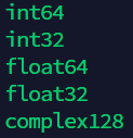
a = np.array([2,23,4],dtype=np.int)
print(a.dtype)
# int 64
a = np.array([2,23,4],dtype=np.int32)
print(a.dtype)
# int32
a = np.array([2,23,4],dtype=np.float)
print(a.dtype)
# float64
a = np.array([2,23,4],dtype=np.float32)
print(a.dtype)
# float32
a = np.array([1,2,3,4],dtype=np.complex128)  
print(a.dtype)
# complex128

2.2 element data storage type conversion

import numpy as np
# Cast through the astype() method of ndarray
# astype creates a new array, even if it is specified as the same type
# When a floating-point number is converted to an integer, the decimal part is discarded:
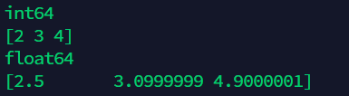
a = np.array([2.5,3.1,4.9],dtype=np.float32)
b = a.astype(np.int64)
print(b.dtype)
print(b)
# If the elements in an array of string type are all numbers, you can also convert them directly to numeric type through this method
a = np.array(["2.5","3.1","4.9"],dtype=np.float32)
b = a.astype(np.float64)
print(b.dtype)
print(b)

3. Conversion between List type and numpy. ndarray type

The array function accepts objects of all sequence types

import numpy as np
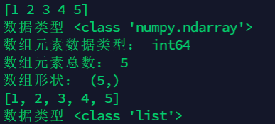
list1 = [1,2,3,4,5] 
#List to numpy.array:
temp = np.array(list1) 
print(temp)
print("data type",type(temp))           #Print array data type  
print("Array element data type:",temp.dtype) #Print array element data type  
print("Total array elements:",temp.size)      #Print array size, that is, the total number of array elements  
print("Array shape:",temp.shape)         #Print array shapes  
#numpy.array to List:
arr = temp.tolist() 
print(arr)
print("data type",type(arr))           #Print array data type

4. Create an array of ndarray

4.1 method 1: list conversion

import numpy as np
#Create array
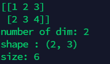
array = np.array([[1,2,3],[2,3,4]])  #List to matrix
print(array)
print('number of dim:',array.ndim)  # dimension
# number of dim: 2
print('shape :',array.shape)    # Number of rows and columns
# shape : (2, 3)
print('size:',array.size)   # Element number
# size: 6

4.2 create special array with zero, ones, empty function

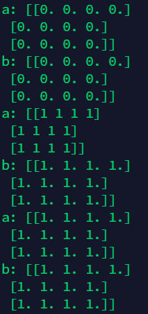
The zeros() function and the ones() function can create an all 0 or all 1 array of a specified length or shape, respectively

The empty() function can create an array of ndarray s without any specific value. It should be noted that the value returned by this function may not be 0, but may be other uninitialized garbage values.

import numpy as np
#Create an all zero array
a = np.zeros((3,4)) # All data are 0, 3 rows and 4 columns
print('a:',a)
b = np.zeros(a.shape) # All data are 0, 3 rows and 4 columns
print('b:',b)
#To create an array, you can also specify the dtype of these specific data:
a = np.ones((3,4),dtype = np.int)   # Data is 1, 3 rows and 4 columns
print('a:',a)
b = np.ones(a.shape) # All data are 0, 3 rows and 4 columns
print('b:',b)
#To create an empty array, each value is close to zero:
a = np.empty((3,4)) # Data is empty, 3 rows and 4 columns
print('a:',a)
b = np.empty(a.shape) # All data are 0, 3 rows and 4 columns
print('b:',b)

4.3 array linspace create linear array

import numpy as np
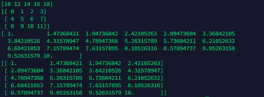
#Use range to create a continuous array:
a = np.arange(10,20,2) # Data of 10-19, 2 steps
print(a)
#Reshape data with reshape
a = np.arange(12).reshape((3,4))    # 3 rows and 4 columns, 0 to 11
print(a)
#Create line segment data with linspace:
a = np.linspace(1,10,20)    # Start end 1 and end end end 10 are divided into 20 data to generate line segments
print(a)
#Also able to do reshape work:
a = np.linspace(1,10,20).reshape((5,4)) # Change shape
print(a)

5. Index and print of matrix

import numpy as np

#One-dimensional index
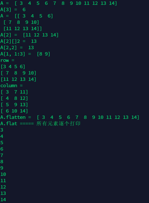
A = np.arange(3,15)
print('A = ',A)
print('A[3] = ',A[3])    # 6

#Two-dimensional
A = np.arange(3,15).reshape((3,4))
print('A = ',A)
print('A[2] = ',A[2])   
print('A[2][]2 = ',A[2][2])     
print('A[2,2] = ',A[2,2])  
print('A[1, 1:3] = ',A[1, 1:3])  

print('row = ')
for row in A:
    print(row)
print('column = ')
for column in A.T:
    print(column)

#flatten is a function of expansion property, which expands the multi-dimensional matrix into one row sequence. And flat is an iterator, itself an object attribute.
print('A.flatten = ',A.flatten())   
print('A.flat ===== Print all elements one by one')  
for item in A.flat:
    print(item)

6. Matrix operation

6.1 basic operation

import numpy as np
array1 = np.array([[1,2,3],[2,3,4]])  #List to matrix
array2 = np.array([[2,3,4],[3,4,5]])  #List to matrix
# subtraction
array3 = array2 - array1
print(array3)
# addition
array3 = array2 + array1
print(array3)
# Multiplication of corresponding elements
array3 = array2 * array1
print(array3)
# Corresponding element multiplication coefficient
array4 = array1 * 2
print(array4)
# Corresponding element power
array4 = array1 ** 2
print(array4)
# Corresponding element sine
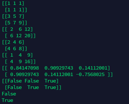
array4 = np.sin(array1)
print(array4)
# Comparison symbol
array5 = array1>2
print(array5)
# Judge whether all matrices are correct
print(array5.all())
# Judge whether the matrix exists correctly
print(array5.any())

6.2 point multiplication

import numpy as np
arr1=np.array([[1,1],[0,1]])
arr2=np.arange(4).reshape((2,2))# deformation
print(arr1)
print(arr2)
# Point multiplication
arr3 = np.dot(arr1,arr2)
print(arr3)

6.3 other matrix characteristic operations

import numpy as np
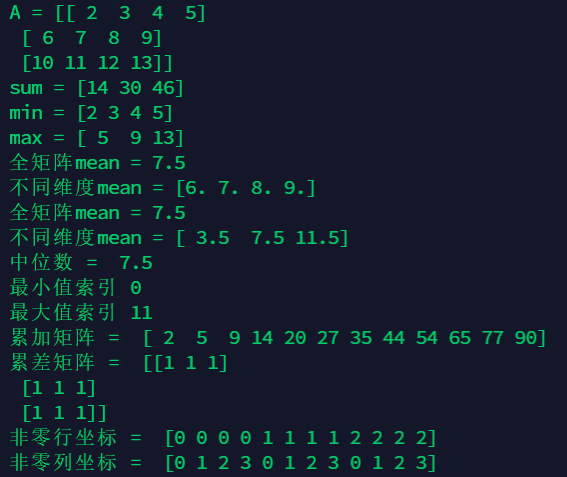
A = np.arange(2,14).reshape((3,4)) 
print("A =",A)
print("sum =",np.sum(A,axis=1))
print("min =",np.min(A,axis=0))
print("max =",np.max(A,axis=1))
print("Full matrix mean =",np.average(A))    
print("Different dimensions mean =",np.average(A,axis=0))    
print("Full matrix mean =",np.mean(A))     
print("Different dimensions mean =",np.mean(A,axis=1))  
print("Median = ",np.median(A))       # 7.5 median
# The two functions argmin() and argmax() respectively correspond to the index of the smallest element and the largest element in the matrix.
# Accordingly, among the 12 elements of the matrix, the minimum value is 2, which corresponds to index 0, the maximum value is 13, and the corresponding index is 11. 
print("Minimum index",np.argmin(A))    # 0
print("Maximum index",np.argmax(A))    # 11
print("Accumulative matrix = ",np.cumsum(A))   #Each element of the matrix generated by the accumulation function (which returns an array) is the sum of the elements added from the first term of the original matrix to the corresponding term
print("Cumulative matrix = ",np.diff(A))    #Cumulative difference operation function
x,y = np.nonzero(A)    #Divide the row and column coordinates of all non-zero elements to form two matrices about row and column respectively
print("Nonzero row coordinates = ",x)
print("Nonzero column coordinates = ",y)

6.3 sorting, transposing and numerical clipping

import numpy as np
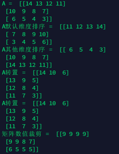
A = np.arange(14,2, -1).reshape((3,4)) 
print("A = ",A)
print("A Default dimension sort = ",np.sort(A))    
print("A Sort other dimensions = ",np.sort(A,axis = 0))    
print("A Transposition = ",np.transpose(A))   #Transposition
print("A Transposition = ",A.T)#Transposition
print("Matrix value clipping = ",np.clip(A,5,9))    #The latter minimum value and maximum value are used to let the function judge whether there are elements smaller than the minimum value or larger than the maximum value in the matrix, and convert these specified elements to the minimum value or maximum value.

7. Other operations

7.1 splicing in transverse and longitudinal direction

import numpy as np
A = np.array([1,1,1])
B = np.array([2,2,2])
# vertical stack merging
C = np.vstack((A,B))
print(C.shape)
print(C)
# horizontal stack merge left and right
D = np.hstack((A,B))       
print(D.shape)
print(D)

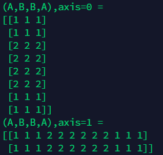
A = np.array([[1,1,1],[1,1,1]])
B = np.array([[2,2,2],[2,2,2]])
C = np.concatenate((A,B,B,A),axis=0)
print("(A,B,B,A),axis=0 = ")
print(C)
D = np.concatenate((A,B,B,A),axis=1)
print("(A,B,B,A),axis=1 = ")
print(D)

7.2 matrix adding or splicing new elements (append or concatenate)

import numpy as np
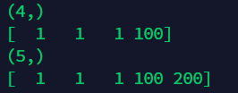
A = np.array([1,1,1])
B = np.concatenate((A,[100])) # First, change p ﹤ to list form for splicing, and note that the input is a tuple
C = np.append(B,200) #Add P directly to p pur_
#Be careful not to forget to cover the original P Φ arr with assignment, otherwise it will not change
print(B.shape)
print(B)
print(C.shape)
print(C)

7.3 add dimension

import numpy as np

#The function of changing dimensions in this way is to transform one-dimensional data into a matrix and multiply it with the weight matrix behind the code. Otherwise, data alone cannot be multiplied in this way.
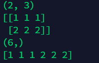
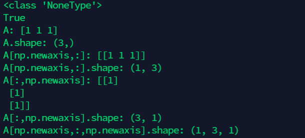
A = np.array([1,1,1])
print(type(np.newaxis))
print(np.newaxis==None)#np.newaxis is equivalent to None in use and function
print("A:",A)
print("A.shape:",A.shape)
print("A[np.newaxis,:]:",A[np.newaxis,:])
print("A[np.newaxis,:].shape:",A[np.newaxis,:].shape)
print("A[:,np.newaxis]:",A[:,np.newaxis])
print("A[:,np.newaxis].shape:",A[:,np.newaxis].shape)
print("A[np.newaxis,:,np.newaxis].shape:",A[np.newaxis,:,np.newaxis].shape)
# (3,1)

7.4 increase / decrease array dimension

import numpy as np
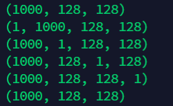
# Suppose the shape of a is [1000128128]
a = np.random.rand(1000,128,128)
print(a.shape)
# Expand? Dims is the dimension whose added content is empty
b=np.expand_dims(a,axis=0)
print(b.shape)
b=np.expand_dims(a,axis=1)
print(b.shape)
b=np.expand_dims(a,axis=2)
print(b.shape)
b=np.expand_dims(a,axis=3)
print(b.shape)
# squeeze is a dimension whose deletion content is empty
c=np.squeeze(b)
print(c.shape)

7.5 slice of matrix

import numpy as np
A = np.arange(12).reshape((3, 4))
print("A = ")
print(A)
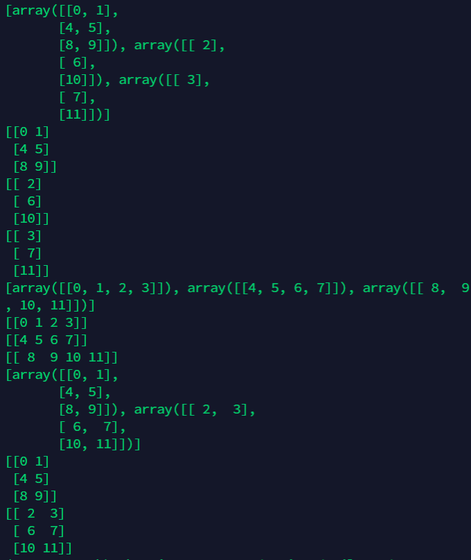
B1,B2 = np.split(A, 2, axis=1)# It returns the array matrix after slicing the two elements in a list
print(np.split(A, 2, axis=1))
print("B1 = ",B1)
print("B2 = ",B2)
C1,C2,C3 = np.split(A, 3, axis=0)
print(np.split(A, 3, axis=0))
print("C1 = ",C1)
print("C2 = ",C2)
print("C3 = ",C3)

import numpy as np
A = np.arange(12).reshape((3, 4))
D1,D2,D3 = np.array_split(A, 3, axis=1)
print(np.array_split(A, 3, axis=1))
print(D1)
print(D2)
print(D3)
E1,E2,E3 = np.vsplit(A, 3) # Longitudinal cutting
print(np.vsplit(A, 3))
print(E1)
print(E2)
print(E3)
F1,F2 = np.hsplit(A, 2) # Horizontal cutting
print(np.hsplit(A, 2)) 
print(F1)
print(F2)

7.6 reshape, t ravel, flatten, post, shape, resize

import numpy as np

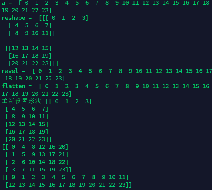
a = np.arange(24)
print('a = ',a)
b = a.reshape(2,3,4)
print('reshape = ',b)
# The t ravel function flattens (that is, changes back to one dimension) a multidimensional array
c = b.ravel()
print('ravel = ',c)
# The flatten function also flattens the multidimensional array, which has the same function as the travel function. However, the flatten function requests to allocate memory to save the result, while the travel function only returns a view of the array
c = b.flatten()
print('flatten = ',c)
# This will directly change the array being manipulated
b.shape = (6,4)
print('Reshape',b)
# transpose function transposes matrix
d = b.transpose()
print("Transposition = ",d)
# The resize function has the same function as the reshape function, but resize directly modifies the array it operates on
# And this step can not be realized by assignment, as shown below
b.resize((2,12))
print('resize Reshape',b)

8. Common operations

8.1 square sum of elements

np.sum(arrayname**2)

8.2 transform numpy to tensorflow's tensor

import numpy as np
import tensorflow as tf
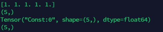
numpy_test = np.ones(5)
print(numpy_test)
print(numpy_test.shape)
tensor_test = tf.convert_to_tensor(numpy_test)
print(tensor_test)
print(tensor_test.shape)