The algorithm of python Development & data structure

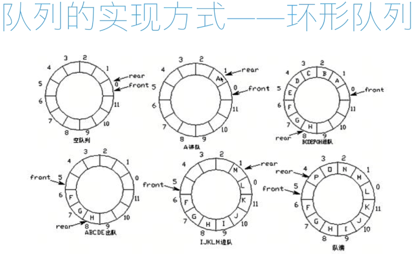
Circular queue: when the pointer = = Maxsize-1, another advance position will automatically reach 0.
Team head pointer forward 1: front = (front + 1)% maxsize
End of team pointer forward 1: rear = (rear + 1)% maxsize
Air condition: rear == front
Team full condition: (rear + 1)% maxsize = = front

class Queue:
    def __init__(self,size=100):
        self.queue = [0 for _ in range(size)]
        self.size = size
        self.rear = 0   # End of line pointer
        self.front = 0   # Team leader pointer

    def push(self, element):
        if not self.is_filled():
            self.rear = (self.rear + 1)%self.size
            self.queue[self.rear] = element
        else:
            raise IndexError("Queue is filled")

    def pop(self):
        if not self.is_empty():
            self.front = (self.front+1) % self.size
            return self.queue[self.front]
        else:
            raise IndexError("Queue is empty")

    # Judge team empty
    def is_empty(self):
        return self.rear == self.front

    # Judge team full
    def is_filled(self):
        return (self.rear+1) % self.size == self.front

2. Python queue built-in module

Usage: from collections import deque
Create queue: queue = deque()
Team entry: append()
Out of line: poppleft ()
Two way queue: appendleft()
Two way queue tail out: pop()

3. List

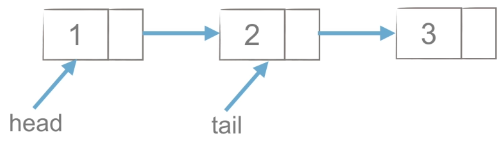
3.1 creating a linked list

Head insertion:

(1) node.next =Head, first point the next of the new node to head.

(2) head = node, and then point the head to the newly added node.

Tail insertion method:

(1) tail.next =Node, first point the next of tail node to the newly added node.

(2) tail = node, and then point the tail to the newly added node.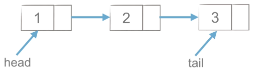

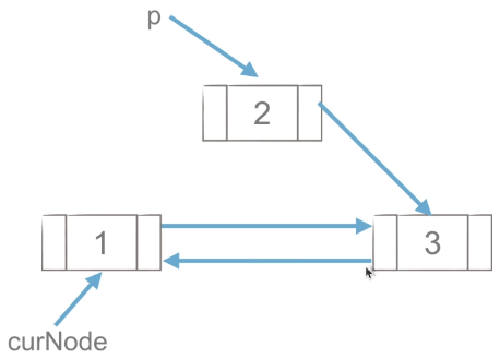
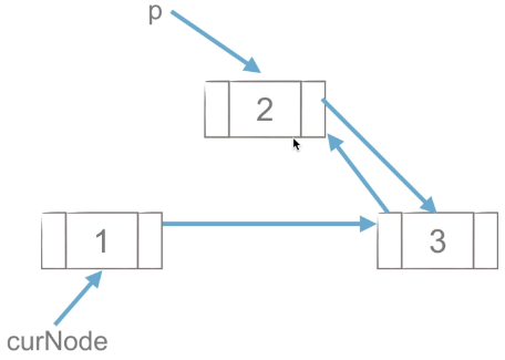
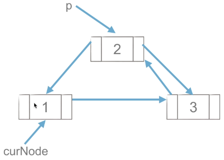
3.2 insertion of linked list nodes

(1)p.next = curNode.next , first point the next of the node to be inserted to the next of the curnode.

(2) curNode.next =p, and then point the next of curnode to the newly added node p.

3.3 deletion of linked list nodes

(1)p = curNode.next

curNode.next =p.next, first point the next of curnode to the next of p.

(2) del p, then delete p.

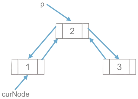
4. Double linked list

4.1 insertion of double linked list nodes

(1)p.next = curNode.next , first point the next of P to the next of curnode.

(2) curNode.next.prior =p, and then point the prior of next of curnode to p.

(3) p.prior = curNode, and then point p's prior to curNode.

(4) curNode.next =p, and finally point the next of curnode to p.

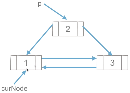
4.2 deletion of bidirectional linked list nodes

(1)p = curNode.next

curNode.next =p.next, first point the next of curnode to the next of p.

(2)p. next.prior =curNode, and then point the prior of the next of P to curNode.

del p, delete p at last.

4.3 chain list and sequence list

The operation of insertion and deletion of linked list is faster than that of sequential list.
The memory of linked list can be allocated more flexibly.
The data structure of linked list is very enlightening to the structure of tree and graph.

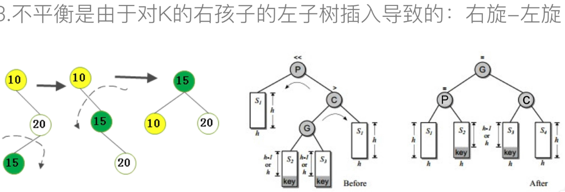
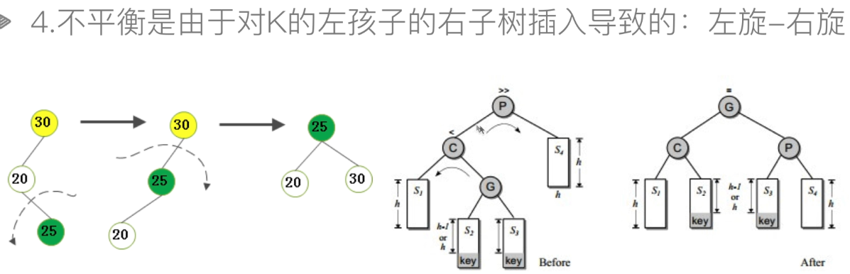
5. AVL tree - rotation

Left hand code:

def rotate_left(self,p,c):
    s2 = c.lchild
    p.child = s2
    if s2:   # To find the parent reversely, you need to judge whether it is empty or not
        s2.parent = p

    c.lchild = p
    p.parent = c

    p.bf = 0
    c.bf = 0
    return c

Right hand code:

def rotate_right(self,p,c):
    s2 = c.rchild
    p.lchild = s2
    if s2:
        s2.parent = p

    c.rchild = p
    p.parent = c

    p.bf = 0
    c.bf = 0
    return c

Right left Code:

def rotate_right_left(self,p,c):
    g = c.lchild
    s3 = g.rchild
    c.lchild = s3
    if s3:
        s3.parent = c
    g.rchild = c
    c.parent = g

    s2 = g.lchild
    p.rchild = s2
    if s2:
        s2.parent = p
    g.lchild = p
    p.parent = g

    # Update bf
    if g.bf > 0:   # Insert at s3
        p.bf = -1
        c.bf = 0
    elif g.bf < 0:   # Insert at s2
        p.bf = 0
        c.bf = 1
    else:   # S1, S2, S3 and S4 are all empty. The inserted one is actually g
        p.bf = 0
        c.bf = 0
    g.bf = 0
    return g

Left right code:

def rotate_left_right(self,p,c):
    g = c.rchild
    s2 = g.lchild
    c.rchild = s2
    if s2:
        s2.parent = c
    g.lchild = c
    c.parent = g

    s3 = g.rchild
    p.lchild = s3
    if s3:
        s3.parent = p
    g.rchild = p
    p.parent = g

    # Update bf
    if g.bf < 0:   # Insert at s2
        p.bf = 1
        c.bf = 0
    elif g.bf > 0:   # Insert at s3
        p.bf = 0
        c.bf = -1
    else:   # S1, S2, S3 and S4 are all empty. The inserted one is actually g
        p.bf = 0
        c.bf = 0
    g.bf = 0
    return g

Extended application of binary search tree - B tree:

algorithm

1. Greedy algorithm

1.1 change problem

Suppose that the shopkeeper needs to change n yuan, and the denomination of the coin is: 100 yuan, 50 yuan, 20 yuan, 5 yuan, 1 yuan. How to change to minimize the number of coins needed?

Code implementation:

# Change question:
t = [100,50,20,5,1]

def change(t,n):
    m = [0 for _ in range(len(t))]
    for i, money in enumerate(t):
        m[i] = n // money
        n = n % money
    return m,n

print(change(t,376))

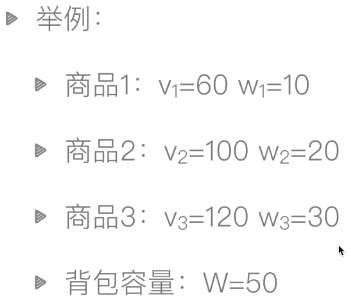
1.2 fractional knapsack problem

Code implementation:

# Fractional knapsack problem:
goods = [(60,10),(100,20),(120,30)]  # Yuan Zu of each commodity (price, weight)
goods.sort(key=lambda x: x[0]/x[1], reverse=True)   # Calculate unit value of goods and sort them from large to small

def fractional_backpack(goods,w):
    m = [0 for _ in range(len(goods))]
    total_v = 0
    for i, (price,weight) in enumerate(goods):
        if w >= weight:
            m[i] = 1
            total_v += price
            w -= weight
        else:
            m[i] = w / weight
            total_v += m[i] * price
            w = 0
            break
    return total_v, m

print(fractional_backpack(goods,50))

1.3 digital splicing

Code implementation:

# Digital splicing:
from functools import cmp_to_key

li = [32,94,128,1286,6,71]

def xy_cmp(x,y):
    if x+y < y+x:
        return 1
    elif x+y > y+x:
        return -1
    else:
        return 0

def number_join(li):
    li = list(map(str,li))
    li.sort(key=cmp_to_key(xy_cmp))
    return "".join(li)

print(number_join(li))

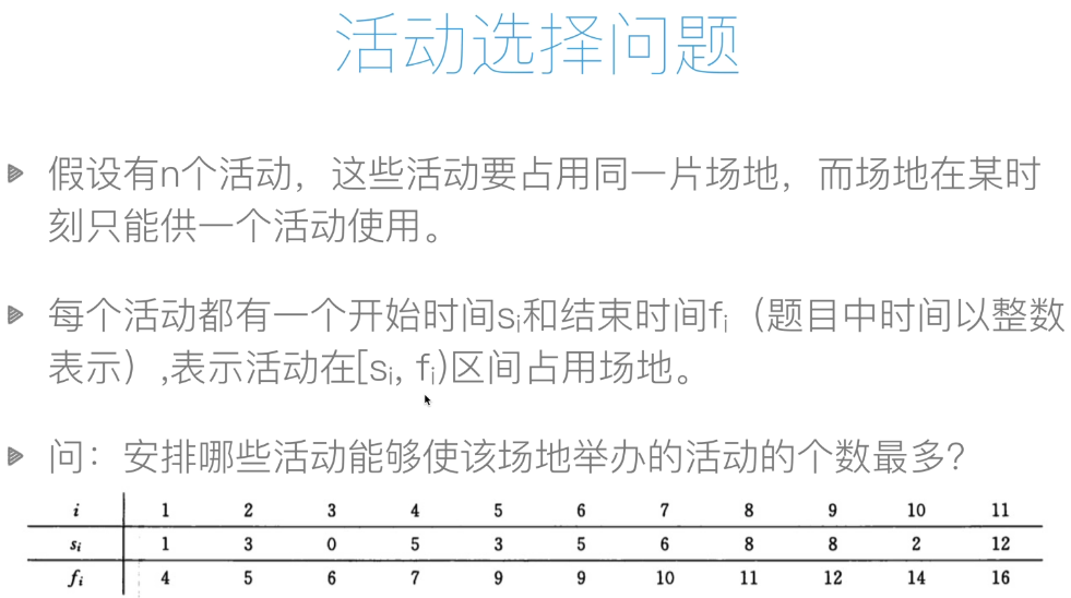
1.4 activity selection

Code implementation:

# Activity selection questions:
activities = [(1,4),(3,5),(0,6),(5,7),(3,9),(5,9),(6,10),(8,11),(8,12),(2,14),(12,16)]
# Ensure activities are ordered by end time
activities.sort(key=lambda x: x[1])

def activity_selection(a):
    res = [a[0]]
    for i in range(1, len(a)):
        if a[i][0] >= res[-1][1]:  # The start time of the current activity is greater than or equal to the end time of the last selected activity
            # No conflict
            res.append(a[i])
    return res

print(activity_selection(activities))

2. Dynamic planning

The key of dynamic programming is to find recurrence!!!

2.1 dynamic planning from Fibonacci series

Code implementation:

# Recursive Fibonacci series: repeated calculation with subproblems, affecting efficiency
def fibnacci(n):
    if n == 1 or n == 2:
        return 1
    else:
        return fibnacci(n-1) + fibnacci(n-2)

# Non recursive Fibonacci series:
# The idea of dynamic programming (DP) = recursive + repetitive subproblem
def fibnacci_no_recurision(n):
    f = [0,1,1]
    if n > 2:
        for i in range(n-2):
            num = f[-1] + f[-2]
            f.append(num)
    return f[n]

print(fibnacci_no_recurision(100))

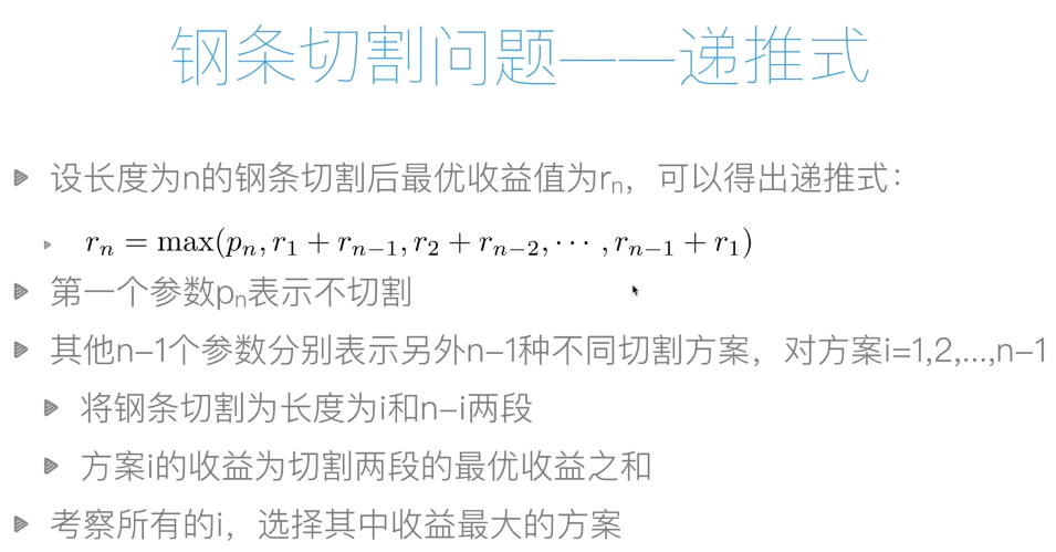
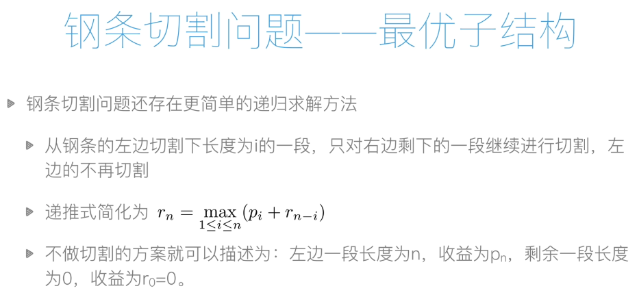
2.2 steel bar cutting

Code implementation:

p = [0,1,5,8,9,10,17,17,20,24,30]

# -----------Top down-------------
# Recursive version 1 steel bar cutting: repeat two sub problems
def cut_rod_recurision_1(p,n):
    if n == 0:
        return 0
    else:
        res = p[0]
        for i in range(1,n):
            res = max(res,cut_rod_recurision_1(p,i) + cut_rod_recurision_1(p, n-i))
        return res


# Recursive version 2 steel bar cutting: repeating a subproblem
def cut_rod_recurision_2(p ,n):
    if n == 0:
        return 0
    else:
        res = 0
        for i in range(1, n+1):
            res = max(res, p[i]+cut_rod_recurision_2(p,n-i))
        return res


# -------------Bottom up--------------
# Dynamic planning version
def cut_rod_dp(p,n):
    r = [0]
    for i in range(1,n+1):
        res = 0
        for j in range(1,i+1):
            res = max(res,p[j]+r[i-j])
        r.append(res)
    return r[n]

Time complexity

The top-down time complexity is: O(2^n)

The bottom-up time complexity is: O(n^2)

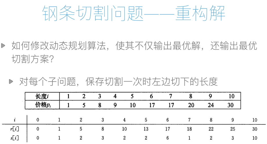
Code implementation:

# ---------Output cutting scheme (where to cut)-----------
def cut_rod_extend(p,n):
    r = [0]
    s = [0]
    for i in range(1,n+1):
        res_r = 0   # Maximum price
        res_s = 0   # The length of the left non cutting part of the scheme corresponding to the maximum price
        for j in range(1,i+1):
            if p[j] + r[i-j] > res_r:
                res_r = p[j] + r[i-j]
                res_s = j
        r.append(res_r)
        s.append(res_s)
    return r[n],s

def cut_rod_solution(p,n):
    r,s = cut_rod_extend(p,n)
    ans = []
    while n > 0:
        ans.append(s[n])
        n -= s[n]
    return ans

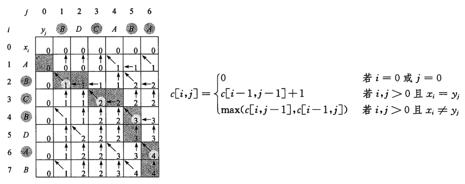
2.3 the longest common subsequence problem

Code implementation:

# ---------Finding the length of the longest common subsequence------------
def lcs_length(x,y):
    m = len(x)
    n = len(y)
    c = [[0 for _ in range(n+1)] for _ in range(m+1)]  # List generation method, generating a (m+1)*(n+1) two-dimensional list
    for i in range(1,m+1):
        for j in range(1,n+1):
            if x[i-1] == y[j-1]:  # When the characters in position i j match, they come from the top left + 1
                c[i][j] = c[i-1][j-1] + 1
            else:
                c[i][j] = max(c[i-1][j],c[i][j-1])
   

# ----------What is the longest subsequence-------------
def lcs(x,y):
    m = len(x)
    n = len(y)
    c = [[0 for _ in range(n+1)] for _ in range(m+1)]
    b = [[0 for _ in range(n+1)] for _ in range(m+1)] # 1: Top left 2: Top 3: left
    for i in range(1,m+1):
        for j in range(1,n+1):
            if x[i-1] == y[j-1]:   # When the characters in position i j match, they come from the top left + 1
                c[i][j] = c[i-1][j-1] + 1
                b[i][j] = 1
            elif c[i-1][j] > c[i][j-1]:   # From above
                c[i][j] = c[i-1][j]
                b[i][j] = 2
            else:
                c[i][j] = c[i][j-1]
                b[i][j] = 3
    return c[m][n], b

# Backtracking: finding the longest subsequence
def lcs_trackback(x,y):
    c,b = lcs(x,y)
    i = len(x)
    j = len(y)
    res = []
    while i > 0 and j > 0:
        if b[i][j] == 1:   # From top left = > match
            res.append(x[i-1])
            i -= 1
            j -= 1
        elif b[i][j] == 2:   # From above = > mismatch
            i -= 1
        else:   # ==3, from left = > mismatch
            j -= 1
    return "".join(reversed(res))

2.4 Euclidean algorithm

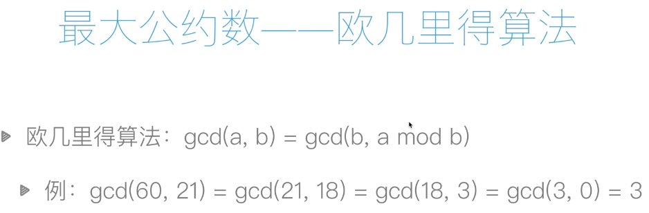
Code implementation:

# Greatest Common Divisor(GCD)
def gcd(a,b):
    if b == 0:
        return a
    else:
        return gcd(b, a % b)

# Finding the greatest common divisor of non recursive version
def gcd2(a,b):
    while b > 0:
        r = a % b
        a = b
        b = r
    return a

Application of Euclidean algorithm: to realize fractional computation

Code implementation:

class Fraction:
    def __init__(self,a,b):
        self.a = a
        self.b = b
        x = self.gcd(a,b)
        self.a /= x
        self.b /= x

    def gcd(self,a, b):
        while b > 0:
            r = a % b
            a = b
            b = r
        return a

    # Least Common Multiple
    def lcm(self,a,b):
        x = self.gcd(a,b)
        return a * b / x

    def __add__(self, other):  # self is a number, the other is another number, find the sum of the two numbers
        a = self.a   # Molecule of the first number
        b = self.b   # First! [insert picture description here]( https://img-blog.csdnimg.cn/2020050617595319.png?x-oss-process=image/watermark,type_ZmFuZ3poZW5naGVpdGk,shadow_10,text_aHR0cHM6Ly9ibG9nLmNzZG4ubmV0L0RyX0JpZ0pvZQ==,size_16,color_FFFFFF,t_70)
//Denominator of number
        c = other.a   # Molecules of the second number
        d = other.b   # Denominator of the second number
        print(a,b,c,d)
        # numerator, denominator
        denominator = self.lcm(b,d)
        numerator = a * denominator / b + c * denominator / d
        return Fraction(numerator,denominator)

    def __str__(self):
        return "%d/%d" % (self.a, self.b)

2.5 RSA encryption algorithm Introduction

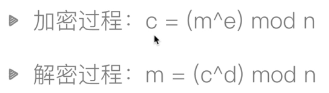
The difficulty of RSA encryption is that it's easy to select two prime numbers for multiplication, but it's difficult to use the number obtained by multiplication to deduce which two prime numbers are multiplied by each other.

==================================================================

See week17 for the code involved

Posted by sm on Thu, 25 Jun 2020 02:27:58 -0700

Programmer Group

The algorithm of python Development & data structure