Text preprocessing

Text is a kind of sequence data. An article can be regarded as a sequence of characters or words. This section will introduce common preprocessing steps of text data, which usually includes four steps:

1. Read in text
2. participle
3. Build a dictionary to map each word to a unique index
4. Convert the text from the sequence of words to the sequence of indexes to facilitate the input of models

Read in text

import collections
import re

def read_time_machine():
    with open('/home/kesci/input/timemachine7163/timemachine.txt', 'r') as f:
        lines = [re.sub('[^a-z]+', ' ', line.strip().lower()) for line in f]
    return lines


lines = read_time_machine()
print('# sentences %d' % len(lines))

With open ('/ home / kesci / input / timemachine7163 / timemachine. TXT','r ') as f: open a text file and create it of type f (iterative);
The strip() method is used to remove the character (space or newline by default) or character sequence specified at the beginning and end of the string;
lower() converts upper case letters to lower case letters;
re.sub(pattern, repl, string, count=0, flags=0)pattern: represents the pattern string in regular expression; repl: the replaced string (either string or function); string: the string to be processed and replaced; count: the number of matches, the default is all replacement; flags: the specific use is unknown.
Therefore, the operation of this read text command is: first remove the space or newline character of each line of text, then change all the uppercase letters in the text to lowercase letters, and finally replace the string of non lowercase letters in the transformed text with spaces.

participle

def tokenize(sentences, token='word'):
    """Split sentences into word or char tokens"""
    if token == 'word':
        return [sentence.split(' ') for sentence in sentences]
    elif token == 'char':
        return [list(sentence) for sentence in sentences]
    else:
        print('ERROR: unkown token type '+token)

tokens = tokenize(lines)
tokens[0:2]

Out[2]
[['the', 'time', 'machine', 'by', 'h', 'g', 'wells', ''], ['']]

This paper defines a function tokenize(sentences, token='word '): sentences is a list, each element in the list is a sentence, token='word'token is a sign, which refers to the level of word segmentation to be made, where word refers to the level of word segmentation to be made; therefore, if word level segmentation is to be made, it is to separate each sentence word with a space character, if it is to be a character Level of participle, directly convert the string to a list.

Segmentation with existing methods

text = "Mr. Chen doesn't agree with my suggestion."

Word segmentation with spaCy method
See you for details. spaCy natural language processing
Create a pipeline by loading the model. Spacy provides many different models, including language information vocabulary, pre trained word vectors, grammar and entities.
The default model English core web will be loaded below. nlp objects will be used to create documents, access language comments and different nlp attributes, which is equivalent to a pipeline, according to which text will be segmented.

import spacy
nlp = spacy.load('en_core_web_sm')
doc = nlp(text)
print([token.text for token in doc])

Output results:

['Mr.', 'Chen', 'does', "n't", 'agree', 'with', 'my', 'suggestion', '.']

Segmentation with NLTK method
In NLTK package, there is a function word "tokenize" for word segmentation. After the text to be segmented is loaded, the word "tokenize" function can be used to complete word segmentation.

from nltk.tokenize import word_tokenize
from nltk import data
data.path.append('/home/kesci/input/nltk_data3784/nltk_data')
print(word_tokenize(text))

Output results:

['Mr.', 'Chen', 'does', "n't", 'agree', 'with', 'my', 'suggestion', '.']

Language model

A natural language text can be regarded as a discrete time series, given a sequence of words w1,w2 ,wTw_1, w_2, \ldots, w_Tw1​,w2​,… , wT, the goal of the language model is to evaluate whether the sequence is reasonable, that is, to calculate the probability of the sequence:
P(w1,w2,...,wT)=∏t=1TP(wt∣w1,...,wt−1)=P(w1)P(w2∣w1)⋯P(wT∣w1w2⋯wT−1) \begin{aligned} P\left(w_{1}, w_{2}, \ldots, w_{T}\right) &=\prod_{t=1}^{T} P\left(w_{t} | w_{1}, \ldots, w_{t-1}\right) \\ &=P\left(w_{1}\right) P\left(w_{2} | w_{1}\right) \cdots P\left(w_{T} | w_{1} w_{2} \cdots w_{T-1}\right) \end{aligned} P(w1​,w2​,...,wT​)​=t=1∏T​P(wt​∣w1​,...,wt−1​)=P(w1​)P(w2​∣w1​)⋯P(wT​∣w1​w2​⋯wT−1​)​
For example, the probability of a text sequence containing four words
P(w1,w2,w3,w4)=P(w1)P(w2∣w1)P(w3∣w1,w2)P(w4∣w1,w2,w3) P\left(w_{1}, w_{2}, w_{3}, w_{4}\right)=P\left(w_{1}\right) P\left(w_{2} | w_{1}\right) P\left(w_{3} | w_{1}, w_{2}\right) P\left(w_{4} | w_{1}, w_{2}, w_{3}\right) P(w1​,w2​,w3​,w4​)=P(w1​)P(w2​∣w1​)P(w3​∣w1​,w2​)P(w4​∣w1​,w2​,w3​)
The parameters of the language model are the probability of words and the conditional probability given the first few words. Suppose the training data set is a large text corpus, such as all items of Wikipedia, the probability of the word can be calculated by the relative word frequency of the word in the training data set, for example, the probability of w1w_1w1 can be calculated as:

P^(w1)=n(w1)n \hat{P}\left(w_{1}\right)=\frac{n\left(w_{1}\right)}{n} P^(w1​)=nn(w1​)​

Where n (W1) n (W1) n (W1) is the number of texts in the corpus with w1w 1 as the first word, and nnn is the total number of texts in the corpus.

Similarly, given the case of w1w, the conditional probability of W2W can be calculated as:

P^(w2∣w1)=n(w1,w2)n(w1) \hat{P}\left(w_{2} | w_{1}\right)=\frac{n\left(w_{1}, w_{2}\right)}{n\left(w_{1}\right)} P^(w2​∣w1​)=n(w1​)n(w1​,w2​)​

Among them, n (W 1, w 2) n (W 1, w 2) n (W 1, w 2) is the number of texts with W 1W 1 as the first word and W 2W 2 as the second word in the corpus.

n meta syntax

With the increase of the length of the sequence, the complexity of calculating and storing the probability of the occurrence of multiple words increases exponentially. 8739w2). Based on the Markov chain of order n − 1n-1n − 1, we can rewrite the language model as

P(w1,w2,...,wT)=∏t=1TP(wt∣wt−(n−1),...,wt−1). P(w_1, w_2, \ldots, w_T) = \prod_{t=1}^T P(w_t \mid w_{t-(n-1)}, \ldots, w_{t-1}) . P(w1​,w2​,...,wT​)=t=1∏T​P(wt​∣wt−(n−1)​,...,wt−1​).

The above is also called n n n grams. It is a probabilistic language model based on N − 1n - 1n − 1-order Markov chain. For example, when n=2n=2n=2, the probability of a text sequence with four words can be rewritten as:
P(w1,w2,w3,w4)=P(w1)P(w2∣w1)P(w3∣w1,w2)P(w4∣w1,w2,w3)=P(w1)P(w2∣w1)P(w3∣w2)P(w4∣w3) \begin{aligned} P\left(w_{1}, w_{2}, w_{3}, w_{4}\right) &=P\left(w_{1}\right) P\left(w_{2} | w_{1}\right) P\left(w_{3} | w_{1}, w_{2}\right) P\left(w_{4} | w_{1}, w_{2}, w_{3}\right) \\ &=P\left(w_{1}\right) P\left(w_{2} | w_{1}\right) P\left(w_{3} | w_{2}\right) P\left(w_{4} | w_{3}\right) \end{aligned} P(w1​,w2​,w3​,w4​)​=P(w1​)P(w2​∣w1​)P(w3​∣w1​,w2​)P(w4​∣w1​,w2​,w3​)=P(w1​)P(w2​∣w1​)P(w3​∣w2​)P(w4​∣w3​)​

When nnn is 1, 2 and 3, we call it unigram, bigram and trigram respectively. For example, the probabilities of sequences W1, w2, w3, w4w 1, w2, w3, w4w1, w2, w3, w4 with length 4 in unary, binary and ternary grammars are respectively
P(w1,w2,w3,w4)=P(w1)P(w2)P(w3)P(w4)P(w1,w2,w3,w4)=P(w1)P(w2∣w1)P(w3∣w2)P(w4∣w3)P(w1,w2,w3,w4)=P(w1)P(w2∣w1)P(w3∣w1,w2)P(w4∣w2,w3) \begin{aligned} &P\left(w_{1}, w_{2}, w_{3}, w_{4}\right)=P\left(w_{1}\right) P\left(w_{2}\right) P\left(w_{3}\right) P\left(w_{4}\right)\\ &P\left(w_{1}, w_{2}, w_{3}, w_{4}\right)=P\left(w_{1}\right) P\left(w_{2} | w_{1}\right) P\left(w_{3} | w_{2}\right) P\left(w_{4} | w_{3}\right)\\ &P\left(w_{1}, w_{2}, w_{3}, w_{4}\right)=P\left(w_{1}\right) P\left(w_{2} | w_{1}\right) P\left(w_{3} | w_{1}, w_{2}\right) P\left(w_{4} | w_{2}, w_{3}\right) \end{aligned} ​P(w1​,w2​,w3​,w4​)=P(w1​)P(w2​)P(w3​)P(w4​)P(w1​,w2​,w3​,w4​)=P(w1​)P(w2​∣w1​)P(w3​∣w2​)P(w4​∣w3​)P(w1​,w2​,w3​,w4​)=P(w1​)P(w2​∣w1​)P(w3​∣w1​,w2​)P(w4​∣w2​,w3​)​

When nnn is small, the nnn meta syntax is often inaccurate.

Language model

Suppose sequence w1,w2 ,wTw_1, w_2, \ldots, w_Tw1​,w2​,… , each word in wT is generated in turn, we have

Language model data set

Read data set

with open('/home/kesci/input/jaychou_lyrics4703/jaychou_lyrics.txt') as f:
    corpus_chars = f.read()
print(len(corpus_chars))
print(corpus_chars[: 40])
corpus_chars = corpus_chars.replace('\n', ' ').replace('\r', ' ')
corpus_chars = corpus_chars[: 10000]

Build character index

idx_to_char = list(set(corpus_chars)) # De duplicate to get index to character mapping
char_to_idx = {char: i for i, char in enumerate(idx_to_char)} # Character to index mapping
vocab_size = len(char_to_idx)
print(vocab_size)

corpus_indices = [char_to_idx[char] for char in corpus_chars]  # Turn each character into an index to get a sequence of indexes
sample = corpus_indices[: 20]
print('chars:', ''.join([idx_to_char[idx] for idx in sample]))
print('indices:', sample)

In list (set (Corpus ﹣ chars)), set() function creates an unordered and unrepeated set of elements, which can be used for relationship testing, deletion of duplicate data, and calculation of intersection, subtraction, union, etc. list() method is used to convert tuples into lists (Note: tuples and lists are very similar, except that the element value of tuples cannot be modified, tuples are placed in brackets, and lists are placed in squares In brackets).
The enumerate() function is used to combine a traversable data object (such as a list, tuple, or string) into an index sequence, listing data and data subscripts at the same time, which is generally used in the for loop. i. Char in enumerate (idx_to_char) is used to enumerate the subscripts of each character and each character.
char: i is the derivation of a dictionary, used to construct a dictionary.
[char_to_idx [char] for char in corpus [char] converts each self reading in corpus into its corresponding index to get an index sequence, and then takes out the first 20 indexes.
[IDX [u to_char [IDX] for IDX in sample]) puts forward the characters corresponding to the index, and join() splices the extracted characters.
The output result is:

1027
chars: Want to have a helicopter want to fly with you to the universe want and
indices: [1022, 648, 1025, 366, 208, 792, 199, 1022, 648, 641, 607, 625, 26, 155, 130, 5, 199, 1022, 648, 641]

Sampling of time series data

Random sampling
The following code randomly samples a small batch of data at a time. Batch size is the number of samples in each small batch, and num steps is the number of time steps in each sample.
In random sampling, each sample is an arbitrary sequence cut from the original sequence, and the positions of two adjacent random small batches on the original sequence are not necessarily adjacent.

import torch
import random
def data_iter_random(corpus_indices, batch_size, num_steps, device=None):
    # Minus 1 is because for a sequence of length N, X contains at most the first n - 1 characters
    num_examples = (len(corpus_indices) - 1) // num_steps  # The number of samples without overlapping is obtained by rounding
    example_indices = [i * num_steps for i in range(num_examples)]  # The subscript of the first character of each sample in corpus  indexes
    random.shuffle(example_indices)

    def _data(i):
        # Returns a sequence of num steps from i
        return corpus_indices[i: i + num_steps]
    if device is None:
        device = torch.device('cuda' if torch.cuda.is_available() else 'cpu')
    
    for i in range(0, num_examples, batch_size):
        # Each time, select batch_size random samples
        batch_indices = example_indices[i: i + batch_size]  # Subscript of the first character of each sample of the current batch
        X = [_data(j) for j in batch_indices]
        Y = [_data(j + 1) for j in batch_indices]
        yield torch.tensor(X, device=device), torch.tensor(Y, device=device)

my_seq = list(range(30))
for X, Y in data_iter_random(my_seq, batch_size=2, num_steps=6):
    print('X: ', X, '\nY:', Y, '\n')

Output:

X:  tensor([[ 6,  7,  8,  9, 10, 11],
        [12, 13, 14, 15, 16, 17]]) 
Y: tensor([[ 7,  8,  9, 10, 11, 12],
        [13, 14, 15, 16, 17, 18]]) 

X:  tensor([[ 0,  1,  2,  3,  4,  5],
        [18, 19, 20, 21, 22, 23]]) 
Y: tensor([[ 1,  2,  3,  4,  5,  6],
        [19, 20, 21, 22, 23, 24]]) 

Adjacent sampling
In adjacent sampling, two adjacent random small batches are adjacent to each other in the original sequence.

def data_iter_consecutive(corpus_indices, batch_size, num_steps, device=None):
    if device is None:
        device = torch.device('cuda' if torch.cuda.is_available() else 'cpu')
    corpus_len = len(corpus_indices) // batch_size * batch_size  # The length of the remaining sequence
    corpus_indices = corpus_indices[: corpus_len]  # Only the first corpus'len characters are reserved
    indices = torch.tensor(corpus_indices, device=device)
    indices = indices.view(batch_size, -1)  # resize into (batch_size,)
    batch_num = (indices.shape[1] - 1) // num_steps
    for i in range(batch_num):
        i = i * num_steps
        X = indices[:, i: i + num_steps]
        Y = indices[:, i + 1: i + num_steps + 1]
        yield X, Y

Under the same setting, print the input X and label Y of small batch samples read each time for adjacent samples. Two adjacent random small batches are adjacent to each other in the original sequence.

for X, Y in data_iter_consecutive(my_seq, batch_size=2, num_steps=6):
    print('X: ', X, '\nY:', Y, '\n')

Output:

X:  tensor([[ 0,  1,  2,  3,  4,  5],
        [15, 16, 17, 18, 19, 20]]) 
Y: tensor([[ 1,  2,  3,  4,  5,  6],
        [16, 17, 18, 19, 20, 21]]) 

X:  tensor([[ 6,  7,  8,  9, 10, 11],
        [21, 22, 23, 24, 25, 26]]) 
Y: tensor([[ 7,  8,  9, 10, 11, 12],
        [22, 23, 24, 25, 26, 27]]) 

Adjacent sampling is related to the structure of cyclic neural network.

Fundamentals of cyclic neural network

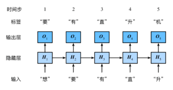
One hot vector

We need to represent the characters as vectors. Here we use the one hot vector. Assuming that the dictionary size is NNN, each character corresponds to a unique index from 000 to N − 1N-1N − 1, then the vector of the character is a vector of NNN length, if the index of the character is iii, then the third position of the vector is 111, and other positions are 000. The one hot vectors with indexes 0 and 2 are shown below. The length of the vectors is equal to the dictionary size.

def one_hot(x, n_class, dtype=torch.float32):
    result = torch.zeros(x.shape[0], n_class, dtype=dtype, device=x.device)  # shape: (n, n_class)
    result.scatter_(1, x.long().view(-1, 1), 1)  # result[i, x[i, 0]] = 1
    return result

In def one hot (x, n class, dtype = torch. Float32), X is a one-dimensional vector, each element of which is an index of a character, and n'class is the size of the dictionary.
scatter() and scatter UU () work the same, except that scatter() does not directly modify the original Tensor, and scatter UU () will. In PyTorch, the underlined function means that there are three parameters to modify scatter(dim, index, src) directly on the original Tensor. Dim: the dimension along which to index; index: the element index used for scatter; src: the source element used for scatter, which can be a scalar or a Tensor.
That is to say, X is an index vector, and the length of X corresponds to the number of rows of the result array. On the first dimension (i.e., row), the x[i] element from the i-row index to scatter is 1, and a one hot two-dimensional array (batch number, dictionary length) is obtained.

The shape of the small batch we sample each time is (batch size, time steps). Because the process of processing small batch is cyclic, that is, processing in time step by step, which is equivalent to processing a column of small batch matrix every time.
The following function transforms such a small batch into several matrices with the shape of (batch size, dictionary size), and the number of matrices equals to the number of time steps. That is to say, the input of time step t t t is Xt ∈ Rn × D \ boldsymbol {x} _t \ in \ matchb {r} ^ {n \ times d} Xt ∈ Rn × D, where nnn is the batch size, ddd is the word vector size, that is, the one hot vector length (Dictionary size).

def to_onehot(X, n_class):
    return [one_hot(X[:, i], n_class) for i in range(X.shape[1])]

X = torch.arange(10).view(2, 5)
inputs = to_onehot(X, vocab_size)
print(len(inputs), inputs[0].shape)

X is the small batch size, and n'u class is the dictionary size. [one hot (x [:, I], n [u class) for I in range (x.shape [1])] takes out a column of batch matrix each time to form a one hot matrix.

Initialize model parameters

num_inputs, num_hiddens, num_outputs = vocab_size, 256, vocab_size
# num_inputs: d
# Num? Hidden: H, the number of hidden cells is a super parameter
# num_outputs: q

def get_params():
    def _one(shape):
        param = torch.zeros(shape, device=device, dtype=torch.float32)
        nn.init.normal_(param, 0, 0.01)
        return torch.nn.Parameter(param)

    # Hide layer parameters
    W_xh = _one((num_inputs, num_hiddens))
    W_hh = _one((num_hiddens, num_hiddens))
    b_h = torch.nn.Parameter(torch.zeros(num_hiddens, device=device))
    # Output layer parameters
    W_hq = _one((num_hiddens, num_outputs))
    b_q = torch.nn.Parameter(torch.zeros(num_outputs, device=device))
    return (W_xh, W_hh, b_h, W_hq, b_q)

Note: Hidden cell is a super parameter!

Definition model

The function rnn completes the calculation of each time step of the recurrent neural network in a cyclic way, that is, the forward calculation of the recurrent neural network.

def rnn(inputs, state, params):
    # Input and output are both num steps and matrix with shape (batch size, vocab size)
    W_xh, W_hh, b_h, W_hq, b_q = params
    H, = state
    outputs = []
    for X in inputs:
        H = torch.tanh(torch.matmul(X, W_xh) + torch.matmul(H, W_hh) + b_h)
        Y = torch.matmul(H, W_hq) + b_q
        outputs.append(Y)
    return outputs, (H,)

#Input and output are both num steps in shape (batch size, vocab size): a matrix in shape (batch size, vocab size) only represents a column in the batch, which can be understood as having n rows of statements. This matrix only represents a column character of the statement matrix, while the statement is a time sequence, and the statement length is the time step, so both input and output are time steps Step matrix, i.e. input and output are all num steps, which are matrix with the shape of (batch size, vocab size).
State is a tuple, in fact, there is only one state in rnn model, that is, hidden state. However, there is more than one state in the subsequent introduction of LSTM, so state is defined as a tuple here.

The init RNN state function initializes the hidden variable, where the return value is a tuple.

def init_rnn_state(batch_size, num_hiddens, device):
    return (torch.zeros((batch_size, num_hiddens), device=device), )

This function finally returns a tuple for the same reason.

Clipping gradient

The gradient of the recurrent neural network is obtained by back propagation, the result is a power form, and the exponent of power is the number of time steps. Therefore, gradient attenuation or gradient explosion are more likely to occur in the recurrent neural network, which will lead to the network almost unable to train. clip gradient is a method to deal with gradient explosion. Suppose we splice the gradients of all model parameters into a vector g\boldsymbol{g}g, and set the clipping threshold to be θ \ theta θ. Cropped gradient

min⁡(θ∥g∥,1)g \min\left(\frac{\theta}{\|\boldsymbol{g}\|}, 1\right)\boldsymbol{g} min(∥g∥θ​,1)g

The L2L norm of does not exceed θ \ theta θ.

def grad_clipping(params, theta, device):
    norm = torch.tensor([0.0], device=device)
    for param in params:
        norm += (param.grad.data ** 2).sum()
    norm = norm.sqrt().item()
    if norm > theta:
        for param in params:
            param.grad.data *= (theta / norm)

Define prediction function

The following function predicts the next num? Chars characters based on the prefix prefix prefix (a string of several characters). This function is a little complex, in which we set rnn as a function parameter, so that we can use this function repeatedly when we introduce other recurrent neural networks in the next section.

def predict_rnn(prefix, num_chars, rnn, params, init_rnn_state,
                num_hiddens, vocab_size, device, idx_to_char, char_to_idx):
    state = init_rnn_state(1, num_hiddens, device)
    output = [char_to_idx[prefix[0]]]   # output record prefix plus predicted num ﹐ chars characters
    for t in range(num_chars + len(prefix) - 1):
        # Take the output of the previous time step as the input of the current time step
        X = to_onehot(torch.tensor([[output[-1]]], device=device), vocab_size)
        # Calculate output and update hidden state
        (Y, state) = rnn(X, state, params)
        # The next time step is to input the characters in the prefix or the current best prediction character
        if t < len(prefix) - 1:
            output.append(char_to_idx[prefix[t + 1]])
        else:
            output.append(Y[0].argmax(dim=1).item())
    return ''.join([idx_to_char[i] for i in output])

Given the model parameters and prefix prefix to predict the next characters, the prediction idea is as follows:
First, a hidden state h is obtained by using the prefix of model processing, and the training information about prefix is recorded in the hidden state H. Since the model has predicted the next character when processing the last character of prefix, this prediction can be used as the input of the next time. Repeat this process until the model predicts num﹐chars characters.

Perplexity

We usually use perplexity to evaluate the language model. Recall "softmax regression" The definition of cross entropy loss function. The degree of perplexity is the value obtained by exponential operation of cross entropy loss function. In particular,

• In the best case, the model always predicts the probability of label category as 1, and the degree of confusion is 1;
• In the worst case, the model always predicts the probability of label category as 0, and the degree of confusion is positive and infinite;
• In the baseline case, the probability of all categories predicted by the model is the same, and the degree of confusion is the number of categories.

Obviously, the confusion of any effective model must be less than the number of categories. In this case, the confusion must be less than the dictionary size, vocab? Size.

Define model training function

Compared with the model training function in the previous chapter, the model training function here has the following differences:

1. The evaluation model of perplexity is used.
2. Cut the gradient before iterating the model parameters.
3. Different sampling methods for time series data will lead to different initialization of hidden state.

def train_and_predict_rnn(rnn, get_params, init_rnn_state, num_hiddens,
                          vocab_size, device, corpus_indices, idx_to_char,
                          char_to_idx, is_random_iter, num_epochs, num_steps,
                          lr, clipping_theta, batch_size, pred_period,
                          pred_len, prefixes):
    if is_random_iter:
        data_iter_fn = d2l.data_iter_random
    else:
        data_iter_fn = d2l.data_iter_consecutive
    params = get_params()
    loss = nn.CrossEntropyLoss()

The is random ITER parameter is used to determine which sampling method to use, random sampling or adjacent sampling. The characteristic of adjacent sampling is that two adjacent batches are continuous in training data, so if adjacent sampling is adopted, only the hidden state needs to be initialized at the beginning of each epoch. But this also brings about a problem, that is, in the same epoch, with the increase of batch, the loss function of the model propagates further with respect to the gradient of hidden variables, and the calculation cost is also greater. Therefore, in order to reduce the computation cost, the hidden state is usually separated from the computation graph at the beginning of each batch.

    for epoch in range(num_epochs):
        if not is_random_iter:  # If adjacent sampling is used, the hidden state is initialized at the beginning of epoch
            state = init_rnn_state(batch_size, num_hiddens, device)
        l_sum, n, start = 0.0, 0, time.time()
        data_iter = data_iter_fn(corpus_indices, batch_size, num_steps, device)
        for X, Y in data_iter:
            if is_random_iter:  # If random sampling is used, the hidden state is initialized before each small batch update
                state = init_rnn_state(batch_size, num_hiddens, device)
            else:  # Otherwise, you need to use the detach function to separate the hidden state from the calculation graph
                for s in state:
                    s.detach_()
            # Input is a matrix whose shapes are (batch size, vocab size)
            inputs = to_onehot(X, vocab_size)
            # outputs have num steps matrices with the shape (batch size, vocab size)
            (outputs, state) = rnn(inputs, state, params)
            # After splicing, the shape is (Num ﹐ steps * batch ﹐ size, vocab ﹐ size)
            outputs = torch.cat(outputs, dim=0)
            # The shape of Y is (batch_size, num_steps), which is transformed to
            # The vector of (Num ﹐ steps * batch ﹐ size,) so that it corresponds to the output line one by one
            y = torch.flatten(Y.T)
            # Using cross entropy loss to calculate average classification error
            l = loss(outputs, y.long())
            
            # Gradient Qing 0
            if params[0].grad is not None:
                for param in params:
                    param.grad.data.zero_()
            l.backward()
            grad_clipping(params, clipping_theta, device)  # Clipping gradient
            d2l.sgd(params, lr, 1)  # Because the error has been averaged, the gradient does not need to be averaged
            l_sum += l.item() * y.shape[0]
            n += y.shape[0]

        if (epoch + 1) % pred_period == 0:
            print('epoch %d, perplexity %f, time %.2f sec' % (
                epoch + 1, math.exp(l_sum / n), time.time() - start))
            for prefix in prefixes:
                print(' -', predict_rnn(prefix, pred_len, rnn, params, init_rnn_state,
                    num_hiddens, vocab_size, device, idx_to_char, char_to_idx))

Simple realization of cyclic neural network

Definition model

We use NN. RNN in Python to construct a cyclic neural network. In this section, we focus on the following constructor parameters of nn.RNN:

• input_size - The number of expected features in the input x
• hidden_size – The number of features in the hidden state h
• nonlinearity – The non-linearity to use. Can be either 'tanh' or 'relu'. Default: 'tanh'
• batch_first – If True, then the input and output tensors are provided as (batch_size, num_steps, input_size). Default: False

Here, the batch [first] determines the input shape. We use the default parameter False, and the corresponding input shape is (Num [steps], batch [size, input [size]).

The forward function has the following parameters:

• input of shape (num_steps, batch_size, input_size): tensor containing the features of the input sequence.
• h_0 of shape (num_layers * num_directions, batch_size, hidden_size): tensor containing the initial hidden state for each element in the batch. Defaults to zero if not provided. If the RNN is bidirectional, num_directions should be 2, else it should be 1.
  If h ﹤ 0 is not set, it defaults to 0.

The return value of the forward function is:

• output of shape (num_steps, batch_size, num_directions * hidden_size): tensor containing the output features (h_t) from the last layer of the RNN, for each t.
• h_n of shape (num_layers * num_directions, batch_size, hidden_size): tensor containing the hidden state for t = num_steps.

Now let's construct an nn.RNN instance and use a simple example to see the shape of the output.

rnn_layer = nn.RNN(input_size=vocab_size, hidden_size=num_hiddens)
num_steps, batch_size = 35, 2
X = torch.rand(num_steps, batch_size, vocab_size)
state = None
Y, state_new = rnn_layer(X, state)
print(Y.shape, state_new.shape)

torch.Size([35, 2, 256]) torch.Size([1, 2, 256])

A complete language model based on recurrent neural network is defined.

class RNNModel(nn.Module):
    def __init__(self, rnn_layer, vocab_size):
        super(RNNModel, self).__init__()
        self.rnn = rnn_layer
        self.hidden_size = rnn_layer.hidden_size * (2 if rnn_layer.bidirectional else 1) 
        self.vocab_size = vocab_size
        self.dense = nn.Linear(self.hidden_size, vocab_size)

    def forward(self, inputs, state):
        # inputs.shape: (batch_size, num_steps)
        X = to_onehot(inputs, vocab_size)
        X = torch.stack(X)  # X.shape: (num_steps, batch_size, vocab_size)
        hiddens, state = self.rnn(X, state)
        hiddens = hiddens.view(-1, hiddens.shape[-1])  # hiddens.shape: (num_steps * batch_size, hidden_size)
        output = self.dense(hiddens)
        return output, state

Where X = torch.stack (X) ා X.shape: (Num ﹐ steps, batch ﹐ size, vocab ﹐ size) is used to stack each small batch of data X, i.e. expand by time dimension.
Similarly, we need to implement a prediction function, which is different from the previous one in forward calculation and initialization of hidden state.

def predict_rnn_pytorch(prefix, num_chars, model, vocab_size, device, idx_to_char,
                      char_to_idx):
    state = None
    output = [char_to_idx[prefix[0]]]  # output record prefix plus predicted num ﹐ chars characters
    for t in range(num_chars + len(prefix) - 1):
        X = torch.tensor([output[-1]], device=device).view(1, 1)
        (Y, state) = model(X, state)  # Forward calculation does not need to pass in model parameters
        if t < len(prefix) - 1:
            output.append(char_to_idx[prefix[t + 1]])
        else:
            output.append(Y.argmax(dim=1).item())
    return ''.join([idx_to_char[i] for i in output])

The next step is to implement the training function, where only adjacent samples are used.

def train_and_predict_rnn_pytorch(model, num_hiddens, vocab_size, device,
                                corpus_indices, idx_to_char, char_to_idx,
                                num_epochs, num_steps, lr, clipping_theta,
                                batch_size, pred_period, pred_len, prefixes):
    loss = nn.CrossEntropyLoss()
    optimizer = torch.optim.Adam(model.parameters(), lr=lr)
    model.to(device)
    for epoch in range(num_epochs):
        l_sum, n, start = 0.0, 0, time.time()
        data_iter = d2l.data_iter_consecutive(corpus_indices, batch_size, num_steps, device) # Adjacent sampling
        state = None
        for X, Y in data_iter:
            if state is not None:
                # Use detach function to separate hidden state from calculation graph
                if isinstance (state, tuple): # LSTM, state:(h, c)  
                    state[0].detach_()
                    state[1].detach_()
                else: 
                    state.detach_()
            (output, state) = model(X, state) # output.shape: (num_steps * batch_size, vocab_size)
            y = torch.flatten(Y.T)
            l = loss(output, y.long())
            
            optimizer.zero_grad()
            l.backward()
            grad_clipping(model.parameters(), clipping_theta, device)
            optimizer.step()
            l_sum += l.item() * y.shape[0]
            n += y.shape[0]
        

        if (epoch + 1) % pred_period == 0:
            print('epoch %d, perplexity %f, time %.2f sec' % (
                epoch + 1, math.exp(l_sum / n), time.time() - start))
            for prefix in prefixes:
                print(' -', predict_rnn_pytorch(
                    prefix, pred_len, model, vocab_size, device, idx_to_char,
                    char_to_idx))

Excerpt of exercise knowledge points

• In the process of batch training, the parameters are updated in batches, and the parameters of models in each batch are the same.
• The cyclic neural network uses the same set of parameters to deal with different length sequences, so the number of parameters of the network is independent of the length of the input sequence.
• The value of hidden state cannot be calculated in parallel, and the hidden state of the next time step is obtained based on all previous hidden states.
• The puzzle degree of a random classification model (baseline model) is equal to the number of categories of classification problems, and the puzzle degree of an effective model should be less than the number of categories.
• Different sampling methods will lead to changes in the initialization mode of hidden state. Only at the beginning of each training cycle can adjacent sampling initialize hidden state because two adjacent batches are continuous in the original data. Each sample in random sampling only contains local time series information. Because the samples are incomplete, each batch needs to be reinitialized The state of Tibet.