Article directory
TensorFlow2 learning -- Image Classification
Guide bag
import matplotlib.pyplot as plt
import numpy as np
import pandas as pd
import tensorflow as tf
from sklearn.preprocessing import StandardScaler
Raw data
- Load dataset
# Clothing picture data set
# Training set All, test set
(X_train_all, y_train_all),(X_test, y_test) = tf.keras.datasets.fashion_mnist.load_data()

# Handwritten digit data set mnist
# tf.keras.datasets.mnist.load_data()
- View datasets
# View data dimensions
print(X_train_all.shape)
# View label categories
print(set(y_train_all))
Data mapping
- Single picture data analysis
# Data of one of the pictures
print(X_train_all[0])
- A matrix of 28 * 28 will be printed here
- The value in the matrix represents the gray value of 0-256 (i.e. one pixel representing the picture)
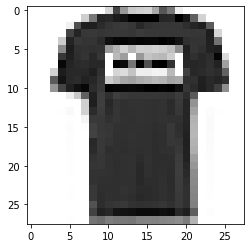
- Show a single picture
def show_single_image(img_arr):
    plt.imshow(img_arr, cmap="binary")
    plt.show()

show_single_image(X_train_all[1])
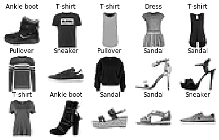
- Show multiple pictures
def show_images(n_rows, n_cols, x_data, y_data, class_names):
    assert len(x_data) == len(y_data)
    assert n_rows * n_cols < len(x_data)

    plt.figure(figsize=(n_cols * 1.5, n_rows * 1.5))
    for row in range(n_rows):
        for col in range(n_cols):
            index = row * n_cols + col
            plt.subplot(n_rows, n_cols, index + 1)
            plt.imshow(x_data[index], cmap="binary", interpolation="nearest")
            plt.axis("off")
            plt.title(class_names[y_data[index]])
    plt.show()

class_names = ["T-shirt", "Trouser", "Pullover", "Dress", "Coat", "Sandal", "Shirt", "Sneaker", "Bag", "Ankle boot"]

show_images(3, 5, X_train_all, y_train_all, class_names)
Data division and standardization
- Split training set and verification set
X_train, X_valid = X_train_all[:50000], X_train_all[50000:]
y_train, y_valid = y_train_all[:50000], y_train_all[50000:]

print("train: ", X_train.shape, y_train.shape)
print("valid: ", X_valid.shape, y_valid.shape)
print(" test: ", X_test.shape, y_test.shape)
- Data standardization
scaler = StandardScaler()
X_train_scaled = scaler.fit_transform(X_train.reshape(-1, 1)).reshape(-1, 28, 28)
X_valid_scaled = scaler.transform(X_valid.reshape(-1, 1)).reshape(-1, 28, 28)
X_test_scaled = scaler.transform(X_test.reshape(-1, 1)).reshape(-1, 28, 28)

print(X_train_scaled.max(), X_train_scaled.min())
Model and train
-
Building neural network layer
# relu: y = max(0, x)
# softmax: it is used to solve the problem of multi classification and change the vector into probability distribution
#          x = [x1, x2, x3]
#          sum = e^x1 + e^x2 + e^x3
#          y = [e^x1/sum, e^x2/sum, e^x3/sum]

# Method 1
# model = tf.keras.models.Sequential()
# model.add(tf.keras.layers.Flatten(input_shape=[28, 28]))
# model.add(tf.keras.layers.Dense(300, activation="relu"))
# model.add(tf.keras.layers.Dense(100, activation="relu"))
# model.add(tf.keras.layers.Dense(10, activation="softmax"))

# Method 2
model = tf.keras.models.Sequential([
    tf.keras.layers.Flatten(input_shape=[28, 28]),
    tf.keras.layers.Dense(200, activation="relu"),
    tf.keras.layers.Dense(150, activation="relu"),
    # tf.keras.layers.Dropout(0.5), # Add a Dropout layer to suppress over fitting. 0.5 means to discard 50% unit
    tf.keras.layers.Dense(100, activation="relu"),
    tf.keras.layers.Dense(10, activation="softmax")
])

# Method 3 functional formula
# input = tf.keras.Input(shape=(28, 28))
# x = tf.keras.layers.Flatten()(input)
# x = tf.keras.layers.Dense(200, activation="relu")(x)
# x = tf.keras.layers.Dense(150, activation="relu")(x)
# x = tf.keras.layers.Dense(100, activation="relu")(x)
# output = tf.keras.layers.Dense(10, activation="softmax")(x)

# model = tf.keras.Model(inputs=input, outputs=output)
- Flatten is used to reduce dimensions. For example, 28 * 28 matrix is broken up into 784 characteristic one-dimensional vectors
- Dense is the full connection layer, receiving all parameters of the previous layer
- The first parameter refers to the number of neuron nodes in this layer
- The second parameter, activation, is the activation function used to process the received data, including relu, sigmoid, softmax, etc
- For the last density, the first parameter is set to 10, because there are only 10 types of data labels, so there are only 10 types of output
-
Model compilation
model.compile(loss = "sparse_categorical_crossentropy",
             optimizer = "adam",
             metrics = ["accuracy"])
- The calculation method of loss function
- For example, it can also be written as mse, category, crossentropy, etc
- Because this is a multi classification problem, you can use sparse ﹣ categorical ﹣ crossentropy or categorical ﹣ crossentropy
- If you want to use the category ﹣ crossentropy, you need to convert the label data to the onehot encoding form. The code is as follows
y_train_onehot = tf.keras.utils.to_categorical(y_train)
y_valid_onehot = tf.keras.utils.to_categorical(y_valid)
y_test_onehot = tf.keras.utils.to_categorical(y_test)
- optimizer represents the way to optimize
- For example, sgd, rmsprop, adam, etc
- It needs to adjust its internal parameters, which can be written as tf.keras.optimizers.Adam(lr=0.001)
- metrics represent the model criteria and will be printed as you train
- The calculation method of loss function
-
Model overview
model.summary()
Model: "sequential_13"
_________________________________________________________________
Layer (type)                 Output Shape              Param #
=================================================================
flatten_13 (Flatten)         (None, 784)               0
_________________________________________________________________
dense_46 (Dense)             (None, 200)               157000
_________________________________________________________________
dense_47 (Dense)             (None, 150)               30150
_________________________________________________________________
dense_48 (Dense)             (None, 100)               15100
_________________________________________________________________
dense_49 (Dense)             (None, 10)                1010
=================================================================
Total params: 203,260
Trainable params: 203,260
Non-trainable params: 0
- Layer column - the network layer we built
- Output Shape column - is the information for the current network layer
- The first parameter, None, is the number of samples, because most of the data will need to be trained when building the model, and so it is None
- The second parameter is the number of neurons in this layer
- Param - is the number of parameters to be trained in the network layer
- Calculation formula: number of nodes in the previous layer * number of nodes in the current layer + number of nodes in the current layer = number of parameters in the current layer
- For example, 784 * 200 + 200 = 1570000200 * 150 + 150 = 30150
- In fact, each node in this layer has a weight w for all nodes in the previous layer. Finally, each node in this layer has an offset value b
-
Start training model
# Training set features
# Y'train is the training set label
# epochs is the number of training batches
# Validation? Data is used to specify the validation set
history = model.fit(X_train_scaled, y_train, epochs=10, validation_data=(X_valid_scaled, y_valid))
- Slow training process, waiting
- Among them, loss: 0.2208 - accuracy: 0.9171 represents the loss value and accuracy of training set
- Where val_loss: 0.3333 - val_accuracy: 0.8916 represents the loss value and accuracy of the validation set
Model evaluation and prediction
- View model training history
pd.DataFrame(history.history)
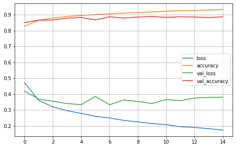
- Drawing with history
pd.DataFrame(history.history).plot(figsize=(8, 5))
plt.grid(True)
#plt.gca().set_ylim(0, 1)
plt.show()
- Model evaluation using test sets
model.evaluate(X_test_scaled, y_test)
- Output result example [0.35619084103703497, 0.8747]
- The first is the loss value and the second is the accuracy rate
- Forecasting with models
- Using predict to predict
# Using predict to predict
result = model.predict(X_test_scaled[0:1])

print(result) # 10 categories, each with a probability
print(result.sum()) # The sum of probability of all categories is 1
print(result.max(), np.argmax(result)) # The most probable is the category of prediction
[[4.1775929e-09 4.8089838e-10 9.2707603e-10 7.3885815e-08 5.2114243e-11
  2.4399082e-03 1.8424946e-09 9.9424636e-03 2.9137237e-12 9.8761755e-01]]
1.0
0.98761755 9
- Use predict class to get the predicted class directly
# Use predict class to get the predicted class directly
print(model.predict_classes(X_test_scaled)[:30])
print(y_test[:30])
[9 2 1 1 6 1 4 6 5 7 4 5 8 3 4 1 2 2 8 0 2 5 7 5 1 2 6 0 9 6]
[9 2 1 1 6 1 4 6 5 7 4 5 7 3 4 1 2 4 8 0 2 5 7 9 1 4 6 0 9 3]
- Using predict to predict
Other: use of Callback
- Callback
- Tensorboard - generate tensorboard records for easy viewing
- EarlyStopping - used to stop training early. If the difference between the local loss and the last loss is less than min_delta, the training will be stopped
- ModelChackpoint - save model, save best only
- Code example
# windows write. / callbacks, linux write. / callbacks, or both (do not specify the forward slash / backslash)
logdir = ".\callbacks"
if not os.path.exists(logdir):
    os.mkdir(logdir)
ouput_model_file = os.path.join(logdir, "fashion_mnist_model.h5")

callbacks = [
    tf.keras.callbacks.TensorBoard(logdir),
    tf.keras.callbacks.ModelCheckpoint(ouput_model_file, save_best_only=True),
    tf.keras.callbacks.EarlyStopping(min_delta=1e-3, patience=5)
]

history = model.fit(X_train_scaled, y_train, epochs=20,
                    validation_data=(X_valid_scaled, y_valid),
                    callbacks = callbacks)
- Check the directory of tensorboard --logdir callbacks

