Fitting curves with rnn

 

Generate the curve point set, X ﹣ ax represents the abscissa, y ﹣ line represents the corresponding ordinate

x_ax = np.linspace(-1, 1, num)


def fun(x):
    #  Is it not very friendly to the square sum exponential function, because the range of values changes too much? Reduce the definition field to - 1,1
    # return 3 * x + 4
    # return np.sin(x)
    # return np.cos(x)
    # return np.sqrt(np.abs(x))
    # return x ** 2

    # Rectangular wave
    y = np.ones_like(x)
    y[np.floor(x) % 2 == 0] = 0
    return y

y_line = fun(x_ax)

Split the point set

#  How many groups, how many in each group
def get_data(batch_size, data_size):
    x = []
    y = []
    for i in range(batch_size):
        s = np.random.randint(0, num - data_size)

        x.append(
            np.array(y_line[s:s + data_size]).reshape((1, data_size))
        )
        y.append(np.array(y_line[s + data_size]).reshape((1, 1)))
    return np.concatenate(x), np.concatenate(y)

 

Effect

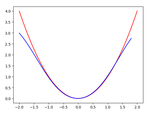
Fit the quadratic function, when the training definition domain is - 1, 1, then expand to - 2, 2 when displaying, and use different intervals, we can find that the effect is still good within - 15, 1.5

 

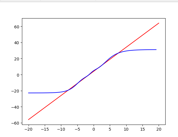
Line prediction

It seems that it is better not to add activation function, but the reason is that the range of value range changes too much

Training - 10, 10, test - 20, 20

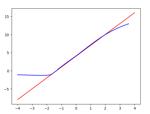
Plus activation function training-2,2, test-4,4

 

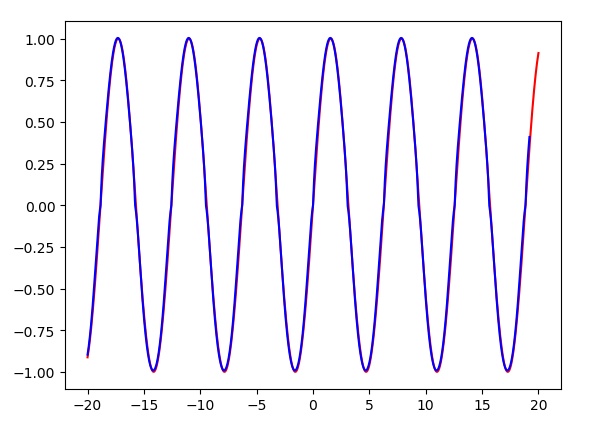
Trigonometric function, for periodic reasons, with a limited range of values, works well

Training - 10, 10, test - 20, 20, almost all fit can be seen

The influence of activation function on trigonometric function is almost not great

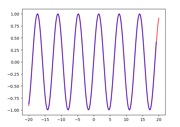
Training-2,2, test-20,20 almost perfect~

 

Rectangular wave

 

Training - 10, 10, test - 20, 20, good results

 

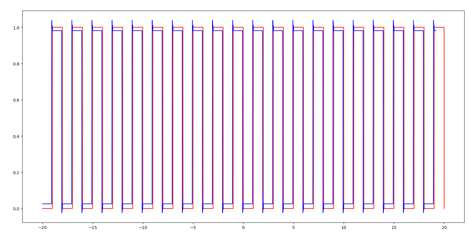
On the whole, rnn is good for the training prediction with periodicity and small variation range, but bad for the monotone sequence.... Maybe we can use a multi-layer and multi time model

It should be able to do time series analysis

import tensorflow as tf
import numpy as np
import matplotlib.pyplot as plt

n_input = 10
lstm_size = 100
n_output = 1
batch_size = 100
train_num = 10000
show_num = 100
num = 1000
# Sequence length
x_ax = np.linspace(-10, 10, num)


# x_ax = np.linspace(-2, 2, num)


def fun(x):
    #  Is it not very friendly to the square sum exponential function, because the range of values changes too much? Reduce the definition field to - 1,1
    # return 3 * x + 4
    # return np.sin(x)
    # return np.cos(x)
    # return np.sqrt(np.abs(x))
    # return x ** 2

    # Rectangular wave
    y = np.ones_like(x)
    y[np.floor(x) % 2 == 0] = 0
    return y


y_line = fun(x_ax)


#  How many groups, how many in each group
def get_data(batch_size, data_size):
    x = []
    y = []
    for i in range(batch_size):
        s = np.random.randint(0, num - data_size)

        x.append(
            np.array(y_line[s:s + data_size]).reshape((1, data_size))
        )
        y.append(np.array(y_line[s + data_size]).reshape((1, 1)))
    return np.concatenate(x), np.concatenate(y)


x_in = tf.placeholder(tf.float32, [None, n_input])
y_in = tf.placeholder(tf.float32, [None, 1])

# Initialization weight
weights = tf.Variable(tf.truncated_normal([lstm_size, n_output], stddev=0.1))
# Initialize offset value
biases = tf.Variable(tf.constant(0.1, shape=[n_output]))


# Define RNN network
def RNN(X, weights, biases):
    inputs = tf.reshape(X, [-1, 1, n_input])
    print(inputs.shape)  # (?, 1, 10)
    # Define LSTM basic CELL
    lstm_cell = tf.contrib.rnn.BasicLSTMCell(lstm_size)
    # outputs is the state of each step
    # final_state[0] is cell state
    # Final state [1] is hidden state equivalent to outputs[-1]
    outputs, final_state = tf.nn.dynamic_rnn(lstm_cell, inputs, dtype=tf.float32)
    print(outputs.shape)  # (?, 1, 100)
    print(final_state[0].shape)  # (?, 100)
    print(final_state[1].shape)  # (?, 100)
    # results = tf.nn.softmax(tf.matmul(final_state[1], weights) + biases)
    results = tf.nn.leaky_relu(tf.matmul(final_state[1], weights) + biases)
    # results = tf.matmul(final_state[1], weights) + biases
    print(results.shape)  # (?, 1)
    return results


# Calculate the return result of RNN
prediction = RNN(x_in, weights, biases)
# loss function
loss = tf.reduce_sum((y_in - prediction) ** 2)
# Optimize with Adam optimizer
train_step = tf.train.AdamOptimizer(1e-4).minimize(loss)
# Initialization
init = tf.global_variables_initializer()

with tf.Session() as sess:
    sess.run(init)
    for epoch in range(train_num):
        batch_xs, batch_ys = get_data(batch_size, n_input)
        sess.run(train_step, feed_dict={x_in: batch_xs, y_in: batch_ys})

        if not (epoch + 1) % show_num:
            batch_xs, batch_ys = get_data(batch_size, n_input)
            acc = sess.run(loss, feed_dict={x_in: batch_xs, y_in: batch_ys})
            print("Iter " + str(epoch + 1) + ", Testing loss= " + str(acc))

    x_ax = np.linspace(-20, 20, num * 5)
    # x_ax = np.linspace(-2, 2, num * 2)
    # x_ax = np.linspace(-4, 4, num * 2)
    y_line = fun(x_ax)

    xx = []
    for i in range(len(y_line) - batch_size):
        # print(i, i + n_input, len(x_line)-batch_size)
        xx.append(
            np.array(y_line[i:i + n_input]).reshape((1, n_input))
        )
    xx = np.concatenate(xx)
    print(xx.shape)
    p = sess.run(
        prediction,
        feed_dict={x_in: xx}
    )
    print(p.shape)
    plt.plot(x_ax[:len(y_line)], y_line, 'r')
    plt.plot(x_ax[:len(p)], p, 'b')
    plt.show()