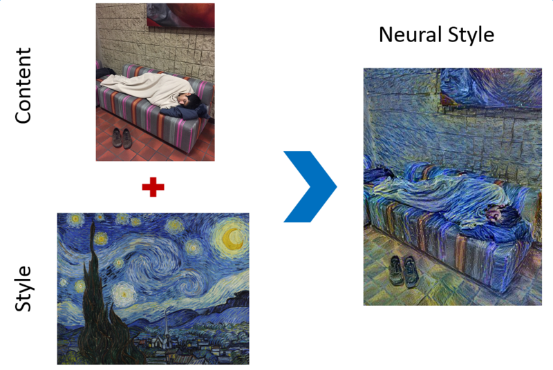
Neural Style is a very interesting in-depth learning application: input a picture of the representative content and a picture of the representative style, and the in-depth learning network will output a new work that combines the style and content.
TensorFlow is Google's most popular open source in-depth learning framework. Author anishathalye implements Neural Style using TensorFlow and puts it open source on GitHub. This paper makes a deep analysis of his code. Please click on the code Here.
Pretrained VGG-19 Model
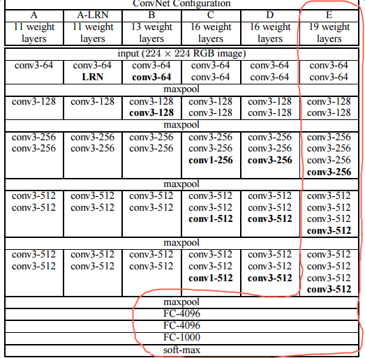
VGG ranked first and second respectively on ILSVRC localization and classification in 2014. VGG-19 is one of the models. The official website provides pre-trained coefficients, which are often used by the industry to transform the features of original pictures.
VGG-19 is a very deep neural network with 19 layers. Its basic structure is as follows:
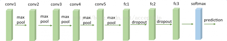
The first several layers are the alternation of convolution and maxpool, each convolution contains several convolution layers, and the last one is followed by three full connection layers. Specifically, the first convolution contains two convolution layers, the second convolution contains two convolution layers, the third convolution contains four convolution layers, the fourth convolution contains four convolution layers, and the fifth convolution contains four convolution layers. Therefore, there are 16 convolution layers, plus three full-connection layers, a total of 19 layers, which is called VGG-19 model. The neural network structure of VGG-19 is shown in the following table:
Neural Style only relies on the convolution layer of VGG-19. Need to use the neural network layer to enumerate as follows:
VGG19_LAYERS = (
    'conv1_1', 'relu1_1', 'conv1_2', 'relu1_2', 'pool1',

    'conv2_1', 'relu2_1', 'conv2_2', 'relu2_2', 'pool2',

    'conv3_1', 'relu3_1', 'conv3_2', 'relu3_2', 'conv3_3',
    'relu3_3', 'conv3_4', 'relu3_4', 'pool3',

    'conv4_1', 'relu4_1', 'conv4_2', 'relu4_2', 'conv4_3',
    'relu4_3', 'conv4_4', 'relu4_4', 'pool4',

    'conv5_1', 'relu5_1', 'conv5_2', 'relu5_2', 'conv5_3',
    'relu5_3', 'conv5_4', 'relu5_4'
)
We can start with MatCovNet Download Page Obtain the model coefficient file of VGG-19 model trained in advance. This file is in Matlab format, and we can use Python's scipy.io to read the data.
This data contains a lot of information. We need information about kernels and bias of each layer of neural network. Kernels are acquired by data['layers'][0] [Layer i] [0] [0] [0] [0] [0] [0] [0] [0] [0] [0] [0] [0], [0] [0] [0] [0], [width, height, in_channels, out_channels], and bias are acquired by data['layers'][0] [0] [Layer i] [0] [0] [0] [0] [0] [0] [0] [0] [0] [0] [0], in the shape of For the convolution of VGG-19, all filters of 3X3 are used, so the width is 3 and the height is 3. Note that the number of layers i refers to the finest-grained layers, including conv, relu, pool, fc operations. Therefore, i=0 is a convolution core, i=1 is a relu, i=2 is a convolution core, i=3 is a relu, i=4 is a pool, i=5 is a convolution core,... i=37 is the full connection layer, and so on. The pooling of VGG-19 uses max-pooling of 2X2 in length and width. Neural Style replaces it with average-pooling, because the author finds that the effect is slightly better.
VGG-19 needs to preprocess the input image in one step, subtracting the RGB mean of each pixel from the training set. The RGB mean of VGG-19 can be obtained by np.mean(data['normalization'][0][0][0], axis=(0, 1), and its value is [123.68 116.779 103.939].
In summary, we can use the following code vgg.py to read the VGG-19 neural network and construct the Neural Style model.
import tensorflow as tf
import numpy as np
import scipy.io

def load_net(data_path):
    data = scipy.io.loadmat(data_path)
    mean = data['normalization'][0][0][0]
    mean_pixel = np.mean(mean, axis=(0,1))
    weights = data['layers'][0]
    return weights, mean_pixel

def net_preloaded(weights, input_image, pooling):
    net = {}
    current = input_image
    for i, name in enumerate(VGG19_LAYERS):
        kind = name[:4]
        if kind == 'conv':
            kernels, bias = weights[i][0][0][0][0]
            # matconvnet: weights are [width, height, in_channels, out_channels]
            # tensorflow: weights are [height, width, in_channels, out_channels]
            kernels = np.transpose(kernels, (1, 0, 2, 3))
            bias = bias.reshape(-1)
            current = _conv_layer(current, kernels, bias)
        elif kind == 'relu':
            current = tf.nn.relu(current)
        elif kind == 'pool':
            current = _pool_layer(current, pooling)
        net[name] = current
    return net

def _conv_layer(input, weights, bias):
    conv = tf.nn.conv2d(input, tf.constant(weights), strides=(1, 1, 1, 1),
            padding='SAME')
    return tf.nn.bias_add(conv, bias)

def _pool_layer(input, pooling):
    if pooling == 'avg':
        return tf.nn.avg_pool(input, ksize=(1, 2, 2, 1), strides=(1, 2, 2, 1),
            padding='SAME')
    else:
        return tf.nn.max_pool(input, ksize=(1, 2, 2, 1), strides=(1, 2, 2, 1),
            padding='SAME')

def preprocess(image, mean_pixel):
    return image - mean_pixel

def unprocess(image, mean_pixel):
    return image + mean_pixel
Neural Style
The core idea of Neural Style is as follows:
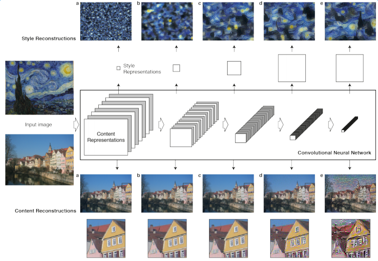
Part 1: Content Reconstruction
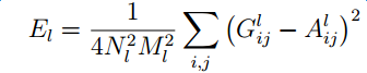
The basic idea is as follows: the content picture p and a randomly generated picture x are transformed through the convolution network of VGG-19 to obtain the feature transformation results of some levels of output, requiring the minimum difference between them. The loss function of the two in layer l is defined as follows:

F_{i j} ^ L is the value of position J for the first convolution core filter of random pictures, and P_{ij}^l is the value of position J for the second convolution core filter of content pictures.
The feature map logic for calculating content pictures is implemented as follows:
# Description of parameters
# network is the path of VGG-19 file
# Content is an array converted from content images
# Pooling as a pooling method

CONTENT_LAYERS = ('relu4_2', 'relu5_2')  # The original paper only uses relu4_2
content_features = {}
shape = (1,) + content.shape  # input shape: [batch, height, width, channels], only one image, so batch=1.

# Obtain the training coefficients of VGG-19 and RGB mean
vgg_weights, vgg_mean_pixel = vgg.load_net(network)


# Computing feature map of Content picture
g = tf.Graph()
with g.as_default(), g.device('/cpu:0'), tf.Session() as sess:
    # Construct Computation Graph, feed as image, output net contains the output of VGG-19 at each level
    image = tf.placeholder('float', shape=shape)
    net = vgg.net_preloaded(vgg_weights, image, pooling)
    # Preprocess content
    content_pre = np.array([vgg.preprocess(content, vgg_mean_pixel)])
    # The content_pre-feed after pretreatment is given to Computation Graph and the calculation results are obtained.
    for layer in CONTENT_LAYERS:
        content_features[layer] = net[layer].eval(feed_dict={image: content_pre})
Calculate the feature map of random pictures and calculate content loss. The logical implementation is as follows:
# Description of parameters
# Image is a randomly generated image
# Pooling as a pooling method
# Content_weight_blend is the ratio of two content reconstruction layers, default is 1, only use more refined reconstruction layer relu4_2; more abstract reconstruction layer relu5_2 is 1-content_weight_blend.
# content_weight is the coefficient of content loss

with tf.Graph().as_default():
    net = vgg.net_preloaded(vgg_weights, image, pooling)
    content_layers_weights = {}
    content_layers_weights['relu4_2'] = content_weight_blend
    content_layers_weights['relu5_2'] = 1.0 - content_weight_blend

    content_loss = 0
    content_losses = []
    for content_layer in CONTENT_LAYERS:
        content_losses.append(content_layers_weights[content_layer] * content_weight * (2 * tf.nn.l2_loss(net[content_layer] - content_features[content_layer]) / content_features[content_layer].size))
        content_loss += reduce(tf.add, content_losses)
Part 2: Style Reconstruction
It's interesting to define what style is mathematically. Each convolution core filter can be regarded as a feature extraction of graphics. Style is simplified in this paper as the correlation of any two features. The description of correlation uses cosine similarity, which is proportional to the dot product of the two features. The mathematical definition of style is then expressed as the dot product of filter i and filter j in the neural network layer, expressed by G_{ij}^l.

Similar to the loss definition in Content Reconstruction, we transform the style image and the randomly generated noise image through the same VGG-19 convolution network to select filters at the specified level. For each level, the difference of $G_{ij}^l $after feature transformation of two images is calculated.
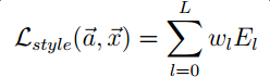
The weighted sum of all levels is the final style loss:
The feature map logic for calculating style pictures is implemented as follows:
# Description of parameters
# styles is a collection of style pictures, which can be multiple pictures
# style_blend_weights are the weights between style picture sets
# style_layers_weights are weights of different neural network layers

STYLE_LAYERS = ('relu1_1', 'relu2_1', 'relu3_1', 'relu4_1', 'relu5_1')
style_shapes = [(1,) + style.shape for style in styles]
style_features = [{} for _ in styles]


# Calculate the feature map of the style picture
for i in range(len(styles)):
    g = tf.Graph()
    with g.as_default(), g.device('/cpu:0'), tf.Session() as sess:
        image = tf.placeholder('float', shape=style_shapes[i])
        net = vgg.net_preloaded(vgg_weights, image, pooling)
        style_pre = np.array([vgg.preprocess(styles[i], vgg_mean_pixel)])
        for layer in STYLE_LAYERS:
            features = net[layer].eval(feed_dict={image: style_pre})
            features = np.reshape(features, (-1, features.shape[3]))  # features.shape[3] is the number of filters
            gram = np.matmul(features.T, features) / features.size
            style_features[i][layer] = gram
The feature map of random pictures is calculated and the logic implementation of style loss is as follows:
# style loss
style_loss = 0
for i in range(len(styles)):
    style_losses = []
    for style_layer in STYLE_LAYERS:
        layer = net[style_layer]
        _, height, width, number = map(lambda i: i.value, layer.get_shape())
        size = height * width * number
        feats = tf.reshape(layer, (-1, number))
        gram = tf.matmul(tf.transpose(feats), feats) / size
        style_gram = style_features[i][style_layer]
        style_losses.append(style_layers_weights[style_layer] * 2 * tf.nn.l2_loss(gram - style_gram) / style_gram.size)
        style_loss += style_weight * style_blend_weights[i] * reduce(tf.add, style_losses)

# tv_loss
# Note: The total variation (TV) loss encourages spatial smoothness in the generated image. It was not used by Gatys et al in their CVPR paper but it can improve the results; for more details and explanation see Mahendran and Vedaldi "Understanding Deep Image Representations by Inverting Them" CVPR 2015.
tv_loss = ...

loss = content_loss + style_loss + tv_loss
train_step = tf.train.AdamOptimizer(learning_rate, beta1, beta2, epsilon).minimize(loss)
The second key file stylize.py of Neural Style TensorFlow code can be obtained by combining the above codes in an orderly manner.