The main function of activation function is to add non-linear factors to solve the problem that linear models can not be multi-classified. It plays a very important role in the whole neural network.
Because the mathematical basis of the neural network is differentiable, the selected activation function should ensure that the data input and output are differentiable.
The activation functions commonly used in neural networks are Sigmoid, Tanh and Relu.

1.Sigmoid function

The mathematical formula of Sigmoid function is

f(x)=11+e−xf(x)=\tfrac{1}{1+e^{-x}}f(x)=1+e−x1​

Using matplotlib to draw the image of Sigmoid function and its derivative

# In matplotlib, by default, there are four axes, two horizontal axes and two vertical axes, which can be obtained by ax=plt.gca().
# gca is the abbreviation of "get current axes", i.e. the axis to get an image. The four axes are top, bottom, left and right, respectively.
# Since axes will get four axes, and we only need two axes, we need to hide the other two axes. After setting the color of the top and right axes to none, the two axes will not be displayed.
# Since we want to draw the image of the Sigmoid function and its derivatives, and we know that the Sigmoid range is (0,1), we set the position of the Y axis to the position of the Sigmoid function y=0 and the position of the X axis to the position of the Sigmoid function x=0.
# 
# 
# plt.legend(loc=?,frameon=?)

# Loc (Set the location of the legend display)
# 'best': 0, (only implemented for axes legends) (adaptive approach)
# 'upper right'  : 1,
# 'upper left'   : 2,
# 'lower left'   : 3,
# 'lower right'  : 4,
# 'right'        : 5,
# 'center left'  : 6,
# 'center right' : 7,
# 'lower center' : 8,
# 'upper center' : 9,
# 'center'       : 10,
# 
# Ncol (set the number of columns to flatten the display, which is useful when there are too many lines to represent)
# 
# 
# 

import math
import numpy as np
import matplotlib.pyplot as plt

x = np.linspace(-10,10,100)  # Generate an isochromatic sequence of x <[-10,10] and length of 100
a = np.array(x)
y1 = 1/(1+math.e**(-a))
y2 = math.e**(-a)/((1+math.e**(-a))**2)
plt.xlim(-11,11)
ax = plt.gca()      
ax.spines['right'].set_color('none')
ax.spines['top'].set_color('none')
ax.xaxis.set_ticks_position('bottom') # Set the position of the x-axis coordinate scale below the x-axis
ax.yaxis.set_ticks_position('left')   # Set the position of the y-axis coordinate scale, above the y-axis
ax.spines['bottom'].set_position(('data',0))
ax.spines['left'].set_position(('data',0))
plt.plot(x,y1,label='Sigmoid',linestyle="-",color="blue")
plt.plot(x,y2,label='Deriv.Sigmoid',linestyle="-",color="red")
plt.legend(['Sigmoid,Deriv.Sigmoid'])               # Show Legend
plt.legend(loc='upper left',frameon=True)  # Frameeon: The default value True is to draw the border, but not if False
plt.show()
# plt.savefig('plot_test.png',dpi=500)

Running results are shown as follows (the blue curve is an image of Sigmoid function, and the red curve is an image of derivative of Sigmoid function)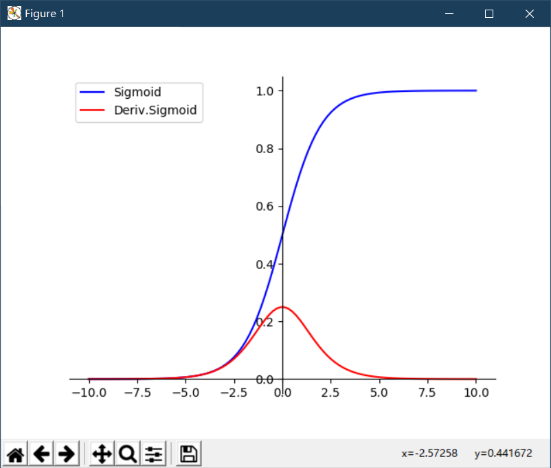

The corresponding function in TensorFlow is

tf.nn.sigmoid(x,name)

The Sigmoid function curve is shown in the figure above, in which the domain of definition is [-, +], but the corresponding range is (0,1). Therefore, the output function of Sigmoid function falls in the range of 0-1.

From an image point of view, as x tends to be positive or negative infinite, the value of y approaches zero or 1, which is called saturation. The function meaning in saturated state, if input a 100 and a 1000, after the Sigmoid function, the response is the same, such a characteristic is equivalent to 1000 more than 100 times the information lost.

From the image of Sigmoid function, it seems that there are obvious gradients when x <[-5,5], but when x exceeds [-5,5], the gradient has gradually disappeared.

2.Tanh function

Tanh function can be said to be a range upgrade version of Sigmoid function, from (0,1) to (1,1). However, Tanh function can not completely replace Simoid function. Sigmoid function is still needed in some cases where the output needs to be greater than 0.

The mathematical formula of Tanh function is

tanh=sinhxcoshx=ex−e−xex+e−xtanh=\frac{sinhx}{coshx}=\frac{e^{x}-e^{-x}}{e^{x}+e^{-x}}tanh=coshxsinhx​=ex+e−xex−e−x​

Using matplotlib to draw the image of Tanh function and its derivative

import math
import numpy as np
import matplotlib.pyplot as plt

x = np.arange(-10,10)
a = np.array(x)
y1 = 2*1/(1+math.e**(-2*a))-1
y2 = 1-(2*1/(1+math.e**(-2*a))-1)**2
plt.xlim(-11,11)
plt.ylim(-1.1,1.1)
ax = plt.gca()      
ax.spines['right'].set_color('none')
ax.spines['top'].set_color('none')
ax.xaxis.set_ticks_position('bottom') # Set the position of the x-axis coordinate scale below the x-axis
ax.yaxis.set_ticks_position('left')   # Set the position of the y-axis coordinate scale, above the y-axis
ax.spines['bottom'].set_position(('data',0))
ax.spines['left'].set_position(('data',0))
plt.plot(x,y1,label='Tanh',linestyle='-',color="blue")
plt.plot(x,y2,label='Deriv Tanh',linestyle='-',color="red")
plt.legend(['Tanh','Deriv Tanh'])               # Show Legend
plt.legend(loc='upper left',frameon=True)  # Frameeon: The default value True is to draw the border, but not if False
plt.show()
# plt.savefig('plot_test.png',dpi=500)

The results are shown in Figure 1 (the blue curve is an image of Tanh function and the red curve is an image of derivative of Tanh function).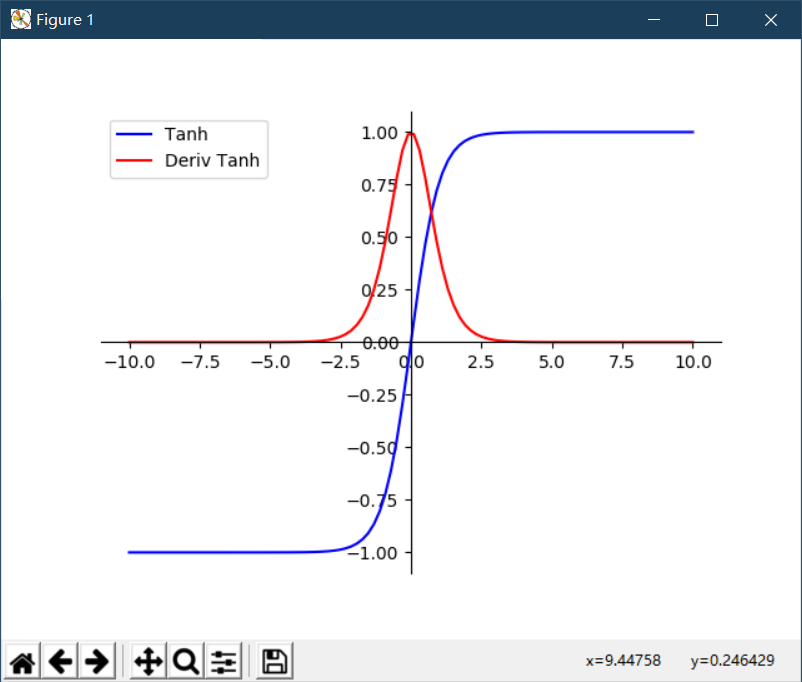

The corresponding function in TensorFlow is

tf.nn.tanh(x,name)

As can be seen from the figure above, Tanh function has the same defect as Sigmoid function and is also a saturation problem. Therefore, when using Tanh function, we should pay attention to the absolute value of input value should not be too large, otherwise the model can not be trained.

3.ReLU function

The mathematical formula of the ReLU function is

f(x)=max(0,x)f(x)=max(0,x)f(x)=max(0,x)

This formula is very simple. If it is greater than 0, it will stay, otherwise it will be zero. ReLU function is widely used because it retains positive signals and ignores negative signals, which is similar to the response of human neurons to signals. So the ReLU function has achieved a good fitting effect in the neural network. In addition, because of the simple operation of ReLU function, it greatly improves the efficiency of machine operation, which is also a great advantage of ReLU function.

Using matplotlib to draw the image of ReLU function and its derivative

import math
import numpy as np
import matplotlib.pyplot as plt

x = np.linspace(-10,10,100)  # Generate an isochromatic sequence of x <[-10,10] and length of 100
a = np.array(x)
y = [i if i>0 else 0 for i in a]
x1 = np.linspace(-10,0,50)
y1 = np.linspace(0,0,50)
x2 = np.linspace(0,10,50)
y2 = np.linspace(1,1,50)
plt.xlim(-11,11)
plt.ylim(-10.1,10.1)
ax = plt.gca()      
ax.spines['right'].set_color('none')
ax.spines['top'].set_color('none')
ax.xaxis.set_ticks_position('bottom') # Set the position of the x-axis coordinate scale below the x-axis
ax.yaxis.set_ticks_position('left')   # Set the position of the y-axis coordinate scale, above the y-axis
ax.spines['bottom'].set_position(('data',0))
ax.spines['left'].set_position(('data',0))
plt.plot(x,y,label='ReLU',linestyle='-',color="blue")
plt.plot(x1,y1,label='Deriv ReLU',linestyle='-',color="red")
plt.plot(x2,y2,label='Deriv ReLU',linestyle='-',color="red")
plt.legend(['ReLU','Deriv ReLU'])               # Show Legend
plt.legend(loc='upper left',frameon=True)  # Frameeon: The default value True is to draw the border, but not if False
plt.show()
# plt.savefig('plot_test.png',dpi=500)

The results of the operation are as follows (the blue curve is the image of ReLU function, and the red curve is the image of ReLU function derivative)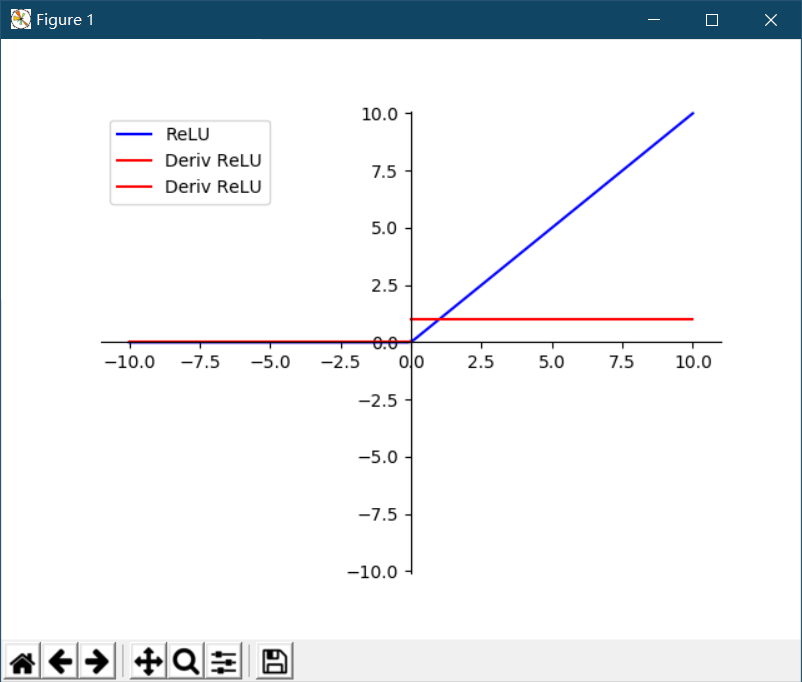

The corresponding function in TensorFlow is

tf.nn.relu(features,name=None) is a general ReLU function, namely max (features, 0)
tf.nn.relu6(features,name=None) is a ReLU function with a threshold of 6, i.e. min (features, 0, 6)

Tips:
The reason why relu6 exists is to prevent gradient explosion. When the number of nodes and layers is very large and the output is positive, their summation is a big value. Especially after several layers of transformation, the final value may be far from the target value. Too large error will lead to too large correction value of parameter adjustment, which will lead to severe network jitter, and ultimately it is difficult to converge.

Similar to the ReLU function is the Softplus function. As shown in the figure below, the difference between the two is that the Softplus function is smoother, but computationally expensive, and retains a little more for values less than 0.

Softplus's mathematical formula is as follows:

f(x)=ln(1+ex)f(x)=ln(1+e^{x})f(x)=ln(1+ex)

Using matplotlib to draw the image of Softplus function and its derivative

import math
import numpy as np
import matplotlib.pyplot as plt

x = np.linspace(-10,10,100)  # Generate an isochromatic sequence of x <[-10,10] and length of 100
a = np.array(x)
y = np.log(1+math.e**a)
y1 = math.e**a/(1+math.e**a)
x_coord = np.linspace(-10,10,21)
y_coord = np.linspace(-10,10,21)
plt.xlim(-11,11)
plt.ylim(-11,11)
plt.xticks(x_coord)
plt.yticks(y_coord)
ax = plt.gca()      
ax.spines['right'].set_color('none')
ax.spines['top'].set_color('none')
ax.xaxis.set_ticks_position('bottom') # Set the position of the x-axis coordinate scale below the x-axis
ax.yaxis.set_ticks_position('left')   # Set the position of the y-axis coordinate scale, above the y-axis
ax.spines['bottom'].set_position(('data',0))
ax.spines['left'].set_position(('data',0))
plt.plot(x,y,label='Softplus',linestyle='-',color="blue")
plt.plot(x,y1,label='Deriv Softplus',linestyle='-',color="red")
plt.legend(['Tanh','Deriv Tanh'])               # Show Legend
plt.legend(loc='upper left',frameon=True)  # Frameeon: The default value True is to draw the border, but not if False
plt.show()
# plt.savefig('plot_test.png',dpi=500)

Screenshots of running results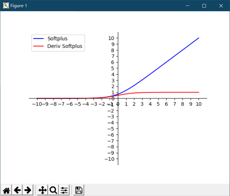

The corresponding function in TensorFlow is

tf.nn.softplus(features,name=None)

Although ReLU function has many advantages in signal response, it is only in forward propagation. Because all the negative values of the model are discarded, it is easy to make the output of the model totally zero so that it can not be trained again. For example, if one of the randomly initialized W-added values is negative, the corresponding positive input value features are all shielded. Similarly, the corresponding negative input value is activated. This is obviously not the result we want.

In addition, as the training proceeds, even if W is positive, if a negative input is multiplied by it, the final result will be adjusted to 0 by the ReLU function filter. This result will lead to the death of neurons in this position, because the gradient of neurons here is 0, which is when the gradient descends later. Nerves in and before this position are not trained to be updated. That is to say, ReLU neurons die irreversibly during training.

Then some variations of functions, such as Leaky ReLU function, have been evolved on the basis of ReLU.

The mathematical formula of Leaky ReLUs function is as follows

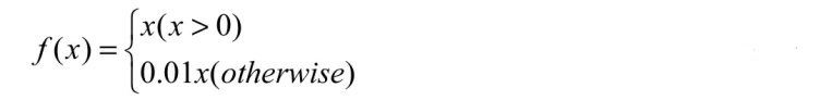
Leaky ReLUs retains some negative values on the basis of ReLU and multiplies x by 0.01. That is to say, Leaky ReLUs does not blindly reject negative signals, but shrinks them.

Then let this 0.01 be the adjustable parameter, so when x is less than 0, multiply a, A is less than or equal to 1. Its mathematical form is as follows

In TensorFlow, the Leaky ReLUs formula does not have a special number, but it can be obtained by using existing functions.

tf.maximum(x,leaky*x,name=name)  # leaky is an incoming parameter

In addition to Leaky ReLUs, there is another function that can also achieve rapid convergence - Elus. When x is less than 0, the Elus function makes a more responsible transformation. The formula is as follows (where alpha is greater than 0)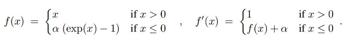

The following are excerpts from Heart of Machine:

Elus is an evolution of ReLU function, which can keep the activation function in a noise-robust state. So an activation function with negative values is proposed, which can make the average activation close to zero, but it will saturate the activation function Elus with smaller parameters as negative values.

Elus function reduces the problem of gradient dispersion by taking the input x itself in the positive interval (1 at the derivative of the interval x > 0), which is characteristic of Relu and Leaky Relu functions. But only the output value of ReLu function has no negative value, so the average value of output will be greater than 0. When the mean value of activation value is not zero, it will cause an bias (offset) to the next layer. If the activation value does not cancel each other (that is, the mean value is not zero), it will cause the activation unit of the next layer to have bias shift. In this way, the more cells there are, the bigger bias shift will be.

Compared with ReLU, Elus can get a negative value, which makes the average activation unit closer to zero, similar to the effect of Batch Normalizatino, but requires less computational complexity. Although Leaky ReLU also has negative values, they do not guarantee robustness to noise in the inactive state (i.e., when the input is negative). On the contrary, Elus has the saturation characteristic when the input value is small, which improves the robustness to noise.

The parameter alpha in the formula is an adjustable parameter, which controls when the negative Elus part saturates.

In TensorFlow, the Elus function corresponds to the following:

tf.nn.relu(features,name=None)

4.Swish function

Swish function is one of the activation functions that Google has found to be more effective than Relu's. The formula is as follows.

f(x)=x×sigmoid(βx)f(x)=x×sigmoid(\beta x)f(x)=x×sigmoid(βx)

Among them, beta beta beta is the zoom parameter of x, which can be chosen by default. In the case of Batch Normalization, it is necessary to adjust the scaling value beta beta beta of X.

Using matplotlib to draw Swish function and its derivative image

import math
import numpy as np
import matplotlib.pyplot as plt

x = np.linspace(-10,10,100)  # Generate an isochromatic sequence of x <[-10,10] and length of 100
a = np.array(x)
y = a * 1/(1+math.e**(-a))  # Let's assume that beta equals 1.
y1 = (1+math.e**(-a)+a*math.e**(-a))/((1+math.e**(-a))**2)
x_coord = np.linspace(-10,10,21)
y_coord = np.linspace(-5,5,11)
plt.xlim(-10,10)
plt.ylim(-5,5)
plt.xticks(x_coord)
plt.yticks(y_coord)
ax = plt.gca()      
ax.spines['right'].set_color('none')
ax.spines['top'].set_color('none')
ax.xaxis.set_ticks_position('bottom') # Set the position of the x-axis coordinate scale below the x-axis
ax.yaxis.set_ticks_position('left')   # Set the position of the y-axis coordinate scale, above the y-axis
ax.spines['bottom'].set_position(('data',0))
ax.spines['left'].set_position(('data',0))
plt.plot(x,y,label='Swish',linestyle='-',color="blue")
plt.plot(x,y1,label='Deriv Swish',linestyle='-',color="red")
plt.legend(['Swish','Deriv Swish'])               # Show Legend
plt.legend(loc='upper left',frameon=True)  # Frameeon: The default value True is to draw the border, but not if False
plt.show()
# plt.savefig('plot_test.png',dpi=500)

Screenshots of running results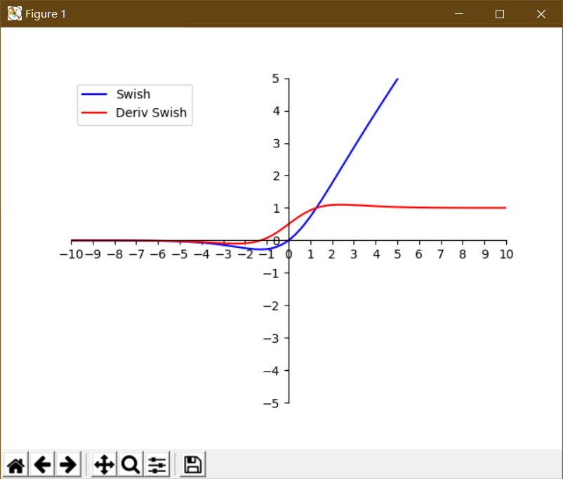

In TensorFlow, there is no separate Swish function, which can be manually encapsulated. The code is as follows:

def Swish(x,beta=1):
	return x * tf.nn.sigmoid(x*beta)

summary

In the neural network, the operation feature is continuous cyclic calculation, so the value of each neuron is constantly changing during each iteration cycle. This leads to the Tanh function's good performance when the feature difference is obvious, and it will expand the feature effect and show it in the process of circulation.

But sometimes when the difference between the calculated features is complex but not obvious, or when the difference between the features is not particularly large, we need a more subtle classification judgment, then the effect of Sigmoid function will be better.

The advantage of the Relu activation function that emerged later is that the data processed by the Relu activation function is more sparse. That is, the data is converted to only the maximum value, and the rest is 0. This transformation can approximately preserve the maximum data characteristics, and is implemented by sparse matrices with most elements of 0.

In fact, the neural network becomes a ReLU function in the process of repeated calculation, trying to express data characteristics with a matrix of most zeros. By using sparse data to express the original data characteristics, the neural network can achieve fast and good results in the iterative operation. So at present, ReLu function is mostly used to replace Sigmoid function.

Reference Books: TensorFlow of Deep Learning: Introduction, Principles and Advanced Practice, by Li Jinhong