The previous article talked about how to build our own network with keras, and explained some common parameters. This article will briefly introduce how to use the framework in the previous article to identify MNIST data sets.

MNIST dataset is already a "chewed" dataset. Many tutorials will "start" on it and almost become a "model"

  We don't need to download from the official website here. When we use this dataset for the first time, it will be automatically downloaded from the official website. Please continue to read it first.

MNIST dataset:
Provide 60000 0-9 handwritten digital pictures and labels with 28 * 28 pixels for training
 Provide 10000 0-9 handwritten digital pictures and labels with 28 * 28 pixels for testing
 Import MNIST MNIST = tf.keras.datasets.mnist
(x_train,y_train),(x_test,y_test) = mnist.load_data()
As an input feature, when the neural network is input, the data is stretched into a one-dimensional array tf.keras.layers.Flatten()

First, let's look at what's in this dataset

import tensorflow as tf
from tensorflow import keras
import matplotlib.pyplot as plt

mnist = keras.datasets.mnist
(x_train,y_train),(x_test,y_test) = mnist.load_data()
print(x_train[0])
print(y_train[0])
for i in range(10):
    plt.imshow(x_train[i])
    plt.show()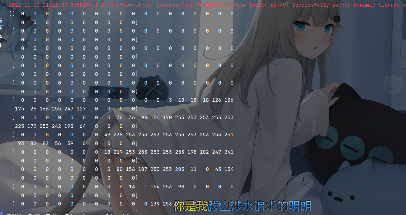

 

 

 

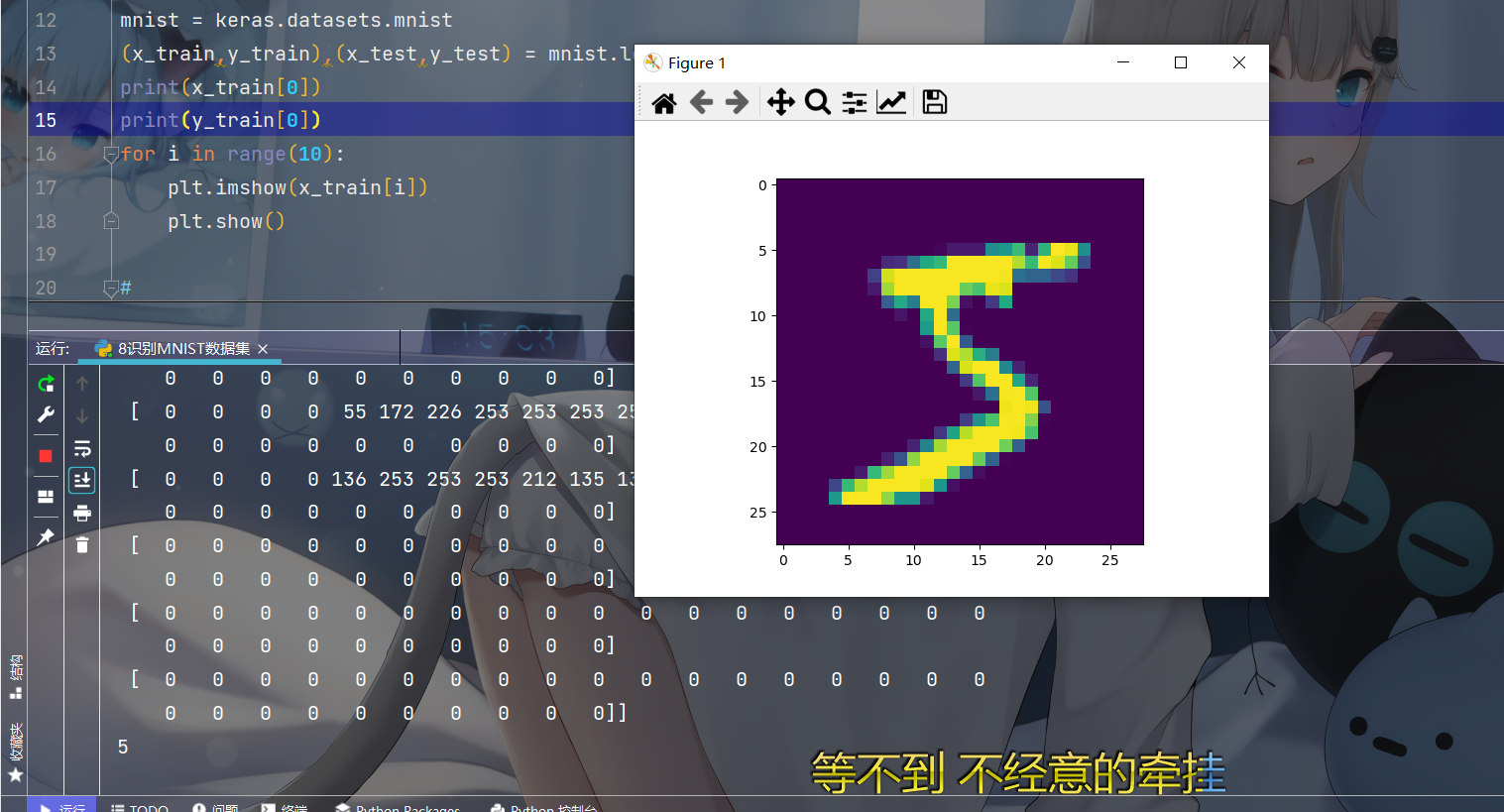
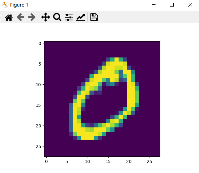
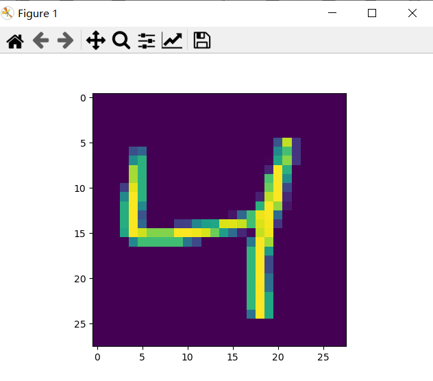
  After the picture is displayed, it is a handwritten numeral picture, and then find a way to deal with this thing

As you can see from the first screenshot, the image value is from 0-255, but this value is a little large during calculation, so let's deal with it a little and reduce it

x_train,x_test = x_train/255.0,x_test/255.0

        Well, it's comfortable now, x_train and X_ Every value in test is between 0-1. After preprocessing, let's start the whole network structure. What did we say in the previous article? Flatten the multidimensional array before processing, so you need to

keras.layers.Flatten() is placed on the first floor

Then, there are 128 neurons in the hidden layer and 10 neurons in the output layer. Because the data set finally identified that there are not 10 numbers, 0-9, so the number of neurons in the output layer is 10. The middle layer, emmmmm and 128, are commonly used. Press it first. I don't know exactly why. If a big man (or giant man) understands, you can leave your answer in the comment area.

The following is the code for network construction

model = keras.models.Sequential([
    keras.layers.Flatten(),
    keras.layers.Dense(128,activation='relu'),
    keras.layers.Dense(10,activation='softmax')
])

By the way, if the last layer is two classification, use sigmoid. If it is multi classification, for example, if there are many output results, use softmax. Little knowledge, get --

Then there is compile. The optimizer selects adam, and the loss function selects losses.SparseCategoricalCrossentropy. These parameter selections can be changed by yourself. Which effect is easy to use. If you don't know other functions, you can make do with me first

After configuration, it's fit training. There's nothing to say. Let's put the complete code below

import tensorflow as tf
from tensorflow import keras
import matplotlib.pyplot as plt

mnist = keras.datasets.mnist
(x_train,y_train),(x_test,y_test) = mnist.load_data()
# print(x_train[0])
# print(y_train[0])
# for i in range(3):
#     plt.imshow(x_train[i])
#     plt.show()

#
x_train,x_test = x_train/255.0,x_test/255.0

model = keras.models.Sequential([
    keras.layers.Flatten(),
    keras.layers.Dense(128,activation='relu'),
    keras.layers.Dense(10,activation='softmax')
])

model.compile(optimizer='adam',
              loss=keras.losses.SparseCategoricalCrossentropy(from_logits=False),
              metrics=['sparse_categorical_accuracy'])

model.fit(x_train,y_train,batch_size=32,epochs=5,validation_data=(x_test,y_test),validation_freq=1)
model.summary()

Run for a while, and the results are shown in the figure

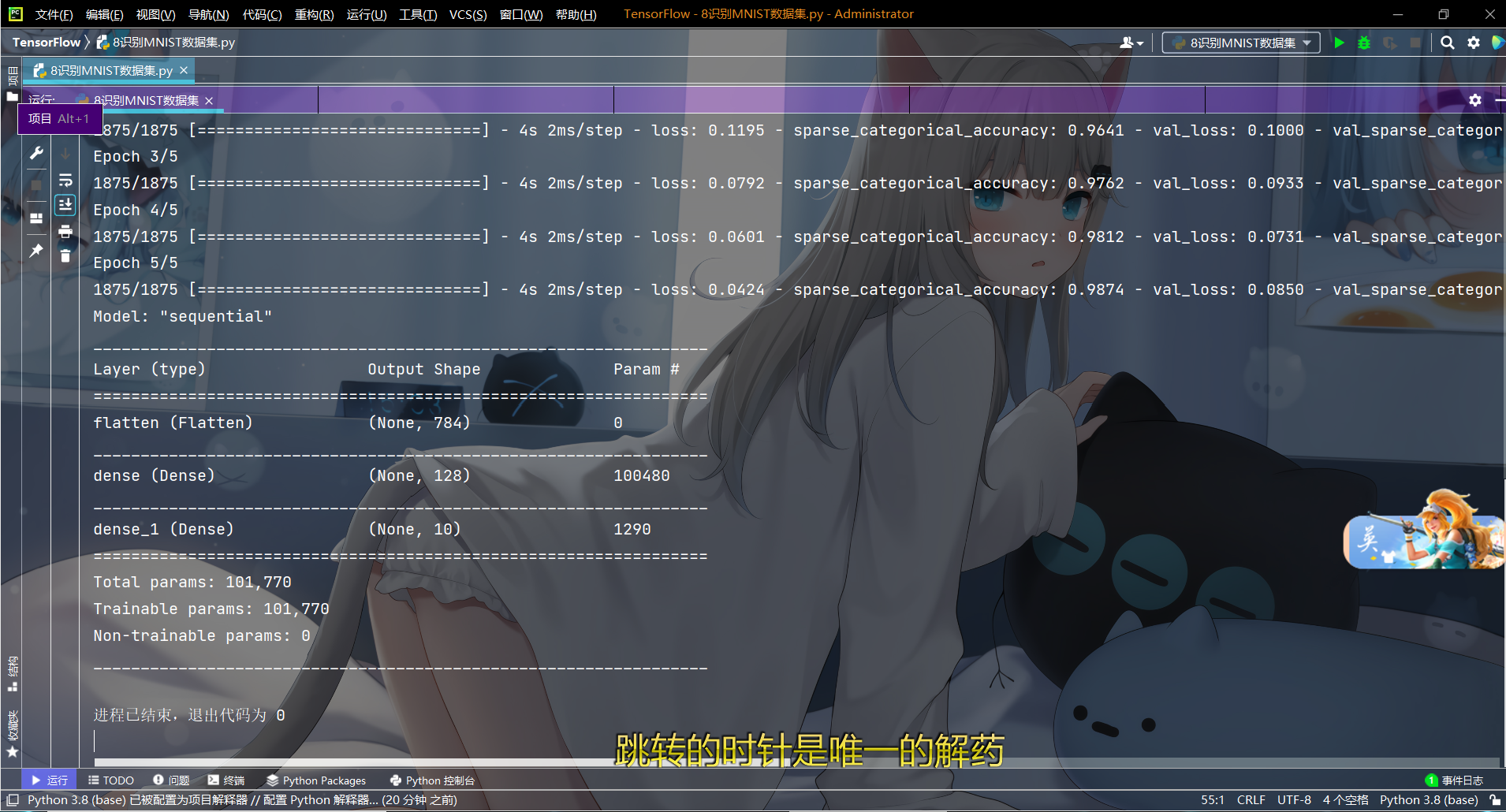
  Accuracy and loss are as follows

  The effect is good, with an accuracy of 0.97. That's all for this article. If you think this article is a little useful for you, give me a free praise. Life is not easy. joker sells art. See you next!