Last time we added an add? Layer function, this time we will create a neural network to predict / fit the corresponding data.
Let's create the following virtual data, which is conic data, but at the same time, some noise is added, and the image is: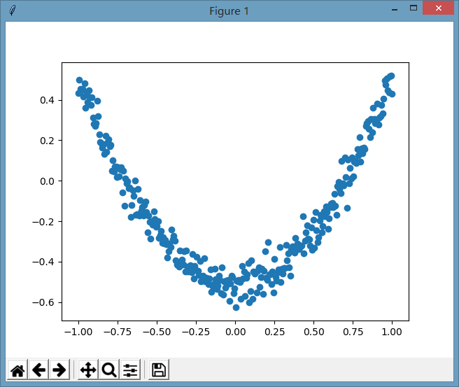
The corresponding code to create these forged data is:
import numpy as np
# Create a column (equivalent to only one attribute value) with an x value of 300 rows. Here, np.newaxis is used to create a new column data with a shape of (300, 1)
x_data = np.linspace(-1, 1, 300)[:,np.newaxis]
# Increase the noise, the mean value of noise is 0, the standard deviation is 0.05, and the shape is the same as that of X ﹐ data
noise = np.random.normal(0, 0.05, x_data.shape)
# Define the function of y as the function of conic, but add some noise data at the same time
y_data = np.square(x_data) - 0.5 + noise
With virtual data, we pretend not to know the laws of this data, so we want to find the laws of these data through a neural network.
This neural network defines a hidden layer and an output layer:
# Define the input value. The purpose of defining the input value here is to make the program more flexible and to receive different actual input values when the neural network is started. The input structure here is that the number of input rows is not fixed, but the column is the value of column 1
xs = tf.placeholder(tf.float32, [None, 1])
ys = tf.placeholder(tf.float32, [None, 1])

# Define a hidden layer. The input is xs and the input size is 1 column. Because there is only one attribute value for X Φ data, we assume that the output neuron has a hidden layer of 10 neurons, and the excitation function uses relu
l1 = add_layer(xs, 1, 10, tf.nn.relu)
# Define the output layer. The input is l1, the input size is 10 columns, that is, the number of columns in l1, and the output size is 1. Because the direct output here is similar to y_data, it is 1 column. Assuming there is no incentive function, that is, what the output is is is directly passed out.
predition = add_layer(l1, 10, 1, activation_function=None)
Then define the loss function as the average of the sum of the squares of the differences
# Define the loss function as the average of the sum of the squares of the differences
loss = tf.reduce_mean(tf.reduce_sum(tf.square(ys - predition), axis=1))
# The gradient descent optimizer is optimized step by step, and the learning efficiency is 0.1. It is optimized by minimizing the loss function
train_step = tf.train.GradientDescentOptimizer(0.1).minimize(loss)
Finally, initialization and training are carried out:
# Initialize all defined variables
init = tf.global_variables_initializer()

sess = tf.Session()
sess.run(init)

# 1000 studies
for i in range(1000):
    sess.run(train_step, feed_dict={xs:x_data, ys:y_data})
    # Error value during printing, see if the error value is decreasing
    if i % 50 == 0:
        print(sess.run(loss, feed_dict={xs:x_data, ys:y_data}))
The complete code is:
import tensorflow as tf


def add_layer(inputs, in_size, out_size, activation_function=None):
    """
    Add layer
    :param inputs: input data
    :param in_size: Number of columns for input data
    :param out_size: Columns of output data
    :param activation_function: Excitation function
    :return:
    """

    # Define the weight, and use random variables at the beginning, which can be simply understood as the random initial point when gradient descent is carried out. This random initial point is better than 0 value, because if it is 0 value, repeated calculation will always be fixed in 0, resulting in the possibility that it will not descend to other positions.
    Weights = tf.Variable(tf.random_normal([in_size, out_size]))
    # Offset shape is 1 row out size column
    biases = tf.Variable(tf.zeros([1, out_size]) + 0.1)
    # Establish the linear formula of neural network: inputs * weights + bias. The transmission of neurons in our brain is basically similar to this linear formula. Here, the weight is the strength coefficient of each neuron transmitting a certain signal. The bias value refers to the original potential value of this neuron
    Wx_plus_b = tf.matmul(inputs, Weights) + biases
    if activation_function is None:
        # If the activation function is not set, the current signal will be directly transmitted intact
        outputs = Wx_plus_b
    else:
        # If the activation function is set, the signal is transferred or suppressed by this activation function
        outputs = activation_function(Wx_plus_b)
    return outputs


import numpy as np
# Create a column (equivalent to only one attribute value) with an x value of 300 rows. Here, np.newaxis is used to create a new column data with a shape of (300, 1)
x_data = np.linspace(-1, 1, 300)[:,np.newaxis]
# Increase the noise, the mean value of noise is 0, the standard deviation is 0.05, and the shape is the same as that of X ﹐ data
noise = np.random.normal(0, 0.05, x_data.shape)
# Define the function of y as the function of conic, but add some noise data at the same time
y_data = np.square(x_data) - 0.5 + noise

# Define the input value. The purpose of defining the input value here is to make the program more flexible and to receive different actual input values when the neural network is started. The input structure here is that the number of input rows is not fixed, but the column is the value of column 1
xs = tf.placeholder(tf.float32, [None, 1])
ys = tf.placeholder(tf.float32, [None, 1])

# Define a hidden layer. The input is xs and the input size is 1 column. Because there is only one attribute value for X Φ data, we assume that the output neuron has a hidden layer of 10 neurons, and the excitation function uses relu
l1 = add_layer(xs, 1, 10, tf.nn.relu)
# Define the output layer. The input is l1, the input size is 10 columns, that is, the number of columns in l1, and the output size is 1. Because the direct output here is similar to y_data, it is 1 column. Assuming there is no incentive function, that is, what the output is is is directly passed out.
predition = add_layer(l1, 10, 1, activation_function=None)

# Define the loss function as the average of the sum of the squares of the differences
loss = tf.reduce_mean(tf.reduce_sum(tf.square(ys - predition), axis=1))
# The gradient descent optimizer is optimized step by step, and the learning efficiency is 0.1. It is optimized by minimizing the loss function
train_step = tf.train.GradientDescentOptimizer(0.1).minimize(loss)

# Initialize all defined variables
init = tf.global_variables_initializer()

sess = tf.Session()
sess.run(init)

# 1000 studies
for i in range(1000):
    sess.run(train_step, feed_dict={xs:x_data, ys:y_data})
    # Error value during printing, see if the error value is decreasing
    if i % 50 == 0:
        print(sess.run(loss, feed_dict={xs:x_data, ys:y_data}))
The output after execution is:
0.558202
0.0136704
0.0095978
0.00769082
0.00639173
0.00552368
0.00489246
0.00448871
0.00421288
0.00402797
0.00389303
0.00378238
0.00370672
0.0036429
0.0035787
0.00350686
0.00344219
0.00338799
0.00332198
0.00326401