Label
background


Once you know the approximate point size, how can it be combined with unmanned driving?
Point clouds are used as location and attribute data in conjunction with auto-driving software.
1. What to use to store point clouds
2. Modeling

Let's first use each record to represent a point (let's talk about optimization later).
1. Table structure (with RDS for PostgreSQL as an example)
create extension postgis;  -- Establish postgis Plug-in unit

postgres=# create table cloudpoint_test(
  id serial primary key,  -- Primary key
  loc geometry,        -- Latitude and longitude(or point)
  other text           -- Other Properties
);
CREATE TABLE
postgres=# create index idx on cloudpoint_test using gist(loc) with (buffering=on);
CREATE INDEX
3. Data writing speed of point clouds
vi ins.sql

insert into cloudpoint_test (loc,other) values (st_makepoint(random()*10000, random()*10000) , 'test');
2.Pour in data performance indicators, about 166,000 records per second.
pgbench -M prepared -n -r -P 1 -f ./ins.sql -c 50 -j 50 -t 2000000

transaction type: Custom query
scaling factor: 1
query mode: prepared
number of clients: 50
number of threads: 50
number of transactions per client: 2000000
number of transactions actually processed: 100000000/100000000
latency average: 0.298 ms
latency stddev: 0.854 ms
tps = 166737.438650 (including connections establishing)
tps = 166739.148413 (excluding connections establishing)
statement latencies in milliseconds:
        0.297896        insert into cloudpoint_test (loc,other) values (st_makepoint(random()*10000, random()*10000) , 'test');
4. Point cloud search design
1. The search point function is as follows
create or replace function ff(geometry, float8, int) returns setof record as $$
declare
  v_rec record;
  v_limit int := $3;
begin
  set local enable_seqscan=off;   -- Forced Index, Scan lines enough to exit.
  for v_rec in
    select *,
    ST_Distance ( $1, loc ) as dist
    from cloudpoint_test
    order by loc <-> $1           -- Return from near to far in distance order
  loop
    if v_limit <=0 then           -- Determine if the number of records returned has reached LIMIT Number of records
      raise notice 'Sufficient limit Set % Bar data, But distance % Points within may also have.', $3, $2;
      return;
    end if;
    if v_rec.dist > $2 then       -- Determine if the distance is greater than the requested distance
      raise notice 'distance % Points within have been output', $2;
      return;
    else
      return next v_rec;
    end if;
    v_limit := v_limit -1;
  end loop;
end;
$$ language plpgsql strict volatile;
postgres=# select * from ff(st_makepoint(1500,1500), 100, 10000) as t (id int, loc geometry, other text, dist float8);
NOTICE:  Sufficient limit 10,000 sets of data, But points within 100 may still exist.
    id     |                    loc                     | other |       dist
-----------+--------------------------------------------+-------+-------------------
  54528779 | 01010000000000EFF6307297400000010D306E9740 | test  | 0.710901366481036
  52422694 | 01010000000080EE51B171974000003DE6256D9740 | test  | 0.829108575682196
  20123322 | 0101000000000074AD5C6F97400000C766CE739740 | test  |   0.9648380442046
  58784192 | 010100000000803A65F4749740008012FDD8709740 | test  |  1.25666215808279
......
5. Search speed of point clouds
1. Search for 200,000 points within 10,000 near st_makepoint(5000,5000) and return from near to far.
explain (analyze,verbose,timing,costs,buffers) select * from ff(st_makepoint(5000,5000), 1000, 200000) as t(id int, loc geometry, other text, dist float8);

NOTICE:  Sufficient limit 200,000 sets of data, But points within 1,000 may still exist.
                                                       QUERY PLAN
------------------------------------------------------------------------------------------------------------------------
 Function Scan on public.ff t  (cost=0.25..10.25 rows=1000 width=76) (actual time=917.748..945.838 rows=200000 loops=1)
   Output: id, loc, other, dist
   Function Call: ff('0101000000000000000088B340000000000088B340'::geometry, 1000::double precision, 200000)
   Buffers: shared hit=201288, temp read=1418 written=1417
 Planning time: 0.057 ms
 Execution time: 959.534 ms
(6 rows)
2. Search for 1 million points within 2000 near st_makepoint(5000,5000) and return from near to far.
explain (analyze,verbose,timing,costs,buffers) select * from ff(st_makepoint(5000,5000), 2000, 1000000) as t(id int, loc geometry, other text, dist float8);

NOTICE:  Sufficient limit 1000000 data sets, But points within 2,000 may still exist.
                                                        QUERY PLAN
---------------------------------------------------------------------------------------------------------------------------
 Function Scan on public.ff t  (cost=0.25..10.25 rows=1000 width=76) (actual time=8867.007..9006.401 rows=1000000 loops=1)
   Output: id, loc, other, dist
   Function Call: ff('0101000000000000000088B340000000000088B340'::geometry, 2000::double precision, 1000000)
   Buffers: shared hit=1006220, temp read=7082 written=7081
 Planning time: 0.059 ms
 Execution time: 9074.267 ms
(6 rows)
explain (analyze,verbose,timing,costs,buffers) select * from ff(st_makepoint(5000,5000), 3000, 5000000) as t(id int, loc geometry, other text, dist float8);

NOTICE:  Sufficient limit 5000000 data sets, But points within 3,000 may still exist.
                                                         QUERY PLAN
-----------------------------------------------------------------------------------------------------------------------------
 Function Scan on public.ff t  (cost=0.25..10.25 rows=1000 width=76) (actual time=42168.038..42861.462 rows=5000000 loops=1)
   Output: id, loc, other, dist
   Function Call: ff('0101000000000000000088B340000000000088B340'::geometry, 3000::double precision, 5000000)
   Buffers: shared hit=5030448, temp read=35402 written=35401
 Planning time: 0.060 ms
 Execution time: 43201.879 ms
(6 rows)
6. Point Cloud Search Bottleneck Analysis
Bottlenecks fall into three categories


perf record -ag -p $PID

perf report -ag --stdio
2. Discrete Scan IO Amplification
3. GiST Index Discreteness Quality
https://www.postgresql.org/docs/10.0/static/gist-implementation.html
Beginning in version 9.2,
PostgreSQL supports a more efficient method to build GiST indexes based on buffering,
which can dramatically reduce the number of random I/Os needed for non-ordered data sets.

For well-ordered data sets the benefit is smaller or non-existent,
because only a small number of pages receive new tuples at a time,
and those pages fit in cache even if the index as whole does not.
How to optimize the above three questions?
7. Point cloud search optimization
1. get next tuple callback optimization
1 Aggregation

The aggregated table structure is designed as follows
postgres=# create table cloudpoint_test_agg(
  id serial primary key,        -- Primary key
  loc_box geometry,          -- lattice(Closed polygon), Represents points within a range
  loc_agg geometry[],        -- Latitude and longitude arrays(or point array)
  other_agg text[]           -- Array of other properties
);
CREATE TABLE

create index idx_cloudpoint_test_agg_1 on cloudpoint_test_agg using gist(loc_box) with (buffering=on);
How do I aggregate?
Art and Technology Value of Honeycomb - PostgreSQL PostGIS's hex-grid
The converted road information is as follows
create table cloudpoint_test_grid(
  id serial primary key,    -- Hexagon ID
  loc_box geometry     -- Single hexagon
);
The JOIN of grid and point cloud data is aggregated into aggregated data.
insert into cloudpoint_test_agg (loc_box,loc_agg,other_agg)
  select t1.loc_box, array_agg(t2.loc) as loc_agg, array_agg(t2.other) as other_agg from
    cloudpoint_test_grid t1 join cloudpoint_test t2
    on (ST_Contains(t1.loc_box, t2.loc)) group by t1.loc_box;
This example uses standard squares for gridding, ((0,0), (10000,10000)) areas are gridded as follows

http://postgis.net/docs/manual-2.3/ST_MakeBox2D.html
do language plpgsql $$
declare
  x int;
  y int;
begin
  for x in select generate_series(0,10000,100) loop
    for y in select generate_series(0,10000,100) loop
      insert into cloudpoint_test_grid(loc_box) values (ST_MakeBox2D( st_makepoint(x,y), st_makepoint(x+100, y+100) ));
    end loop;
  end loop;
end;
$$;
postgres=# select * from cloudpoint_test_grid;
  id   |                                                                                          loc_box
-------+--------------------------------------------------------------------------------------------------------------------------------------------------------------------------------------------
     1 | 010300000001000000050000000000000000000000000000000000000000000000000000000000000000005940000000000000594000000000000059400000000000005940000000000000000000000000000000000000000000000000
     2 | 010300000001000000050000000000000000000000000000000000594000000000000000000000000000006940000000000000594000000000000069400000000000005940000000000000594000000000000000000000000000005940
     3 | 010300000001000000050000000000000000000000000000000000694000000000000000000000000000C0724000000000000059400000000000C072400000000000005940000000000000694000000000000000000000000000006940
     4 | 0103000000010000000500000000000000000000000000000000C07240000000000000000000000000000079400000000000005940000000000000794000000000000059400000000000C0724000000000000000000000000000C07240

......
insert into cloudpoint_test_agg (loc_box,loc_agg,other_agg)
  select t1.loc_box, array_agg(t2.loc) as loc_agg, array_agg(t2.other) as other_agg from
    cloudpoint_test_grid t1 join cloudpoint_test t2
    on (ST_Contains(t1.loc_box, t2.loc)) group by t1.loc_box;

INSERT 0 10000

select count(*) from cloudpoint_test_agg;
10000
The function to search for nearby points from aggregated point cloud data is as follows
create or replace function ff1(geometry, float8, int) returns setof record as $$
declare
  v_rec record;
  v_limit int := $3;
begin
  set local enable_seqscan=off;   -- Forced Index, Scan lines enough to exit.
  for v_rec in
    select *,
    ST_Distance ( $1, loc_box ) as dist
    from cloudpoint_test_agg
    order by loc_box <-> $1           -- Return from near to far in distance order
  loop
    if v_limit <=0 then           -- Determine if the number of records returned has reached LIMIT Number of records
      raise notice 'Sufficient limit Set % Bar data, But distance % Points within may also have.', $3, $2;
      return;
    end if;
    if v_rec.dist > $2 then       -- Determine if the distance is greater than the requested distance
      raise notice 'distance % Points within have been output', $2;
      return;
    else
      return next v_rec;
    end if;
    v_limit := v_limit - array_length(v_rec.loc_agg, 1);  -- Deductions grid Internal point Number
  end loop;
end;
$$ language plpgsql strict volatile;
Example of aggregated search SQL
postgres=# select * from ff1(st_makepoint(1500,1500), 100, 10000) as t (id int, loc_box geometry, loc_agg geometry[], other_agg text[], dist float8);
Aggregated Speed Test
1. Search for 200,000 points within 10,000 near st_makepoint(5000,5000) and return from near to far.
postgres=# explain (analyze,verbose,timing,costs,buffers) select * from ff1(st_makepoint(5000,5000), 1000, 200000) as t (id int, loc_box geometry, loc_agg geometry[], other_agg text[], dist float8);
NOTICE:  Sufficient limit 200,000 sets of data, But points within 1,000 may still exist.
                                                     QUERY PLAN
--------------------------------------------------------------------------------------------------------------------
 Function Scan on public.ff1 t  (cost=0.25..10.25 rows=1000 width=108) (actual time=15.642..15.643 rows=20 loops=1)
   Output: id, loc_box, loc_agg, other_agg, dist
   Function Call: ff1('0101000000000000000088B340000000000088B340'::geometry, 1000::double precision, 200000)
   Buffers: shared hit=465
 Planning time: 0.082 ms
 Execution time: 15.670 ms
(6 rows)
2. Search for 1 million points within 2000 near st_makepoint(5000,5000) and return from near to far.
postgres=# explain (analyze,verbose,timing,costs,buffers) select * from ff1(st_makepoint(5000,5000), 2000, 1000000) as t (id int, loc_box geometry, loc_agg geometry[], other_agg text[], dist float8);
NOTICE:  Sufficient limit 1000000 data sets, But points within 2,000 may still exist.
                                                     QUERY PLAN
---------------------------------------------------------------------------------------------------------------------
 Function Scan on public.ff1 t  (cost=0.25..10.25 rows=1000 width=108) (actual time=63.287..63.296 rows=100 loops=1)
   Output: id, loc_box, loc_agg, other_agg, dist
   Function Call: ff1('0101000000000000000088B340000000000088B340'::geometry, 2000::double precision, 1000000)
   Buffers: shared hit=2143
 Planning time: 0.057 ms
 Execution time: 63.322 ms
(6 rows)
postgres=# explain (analyze,verbose,timing,costs,buffers) select * from ff1(st_makepoint(5000,5000), 3000, 5000000) as t (id int, loc_box geometry, loc_agg geometry[], other_agg text[], dist float8);
NOTICE:  Sufficient limit 5000000 data sets, But points within 3,000 may still exist.
                                                      QUERY PLAN
-----------------------------------------------------------------------------------------------------------------------
 Function Scan on public.ff1 t  (cost=0.25..10.25 rows=1000 width=108) (actual time=312.315..312.394 rows=501 loops=1)
   Output: id, loc_box, loc_agg, other_agg, dist
   Function Call: ff1('0101000000000000000088B340000000000088B340'::geometry, 3000::double precision, 5000000)
   Buffers: shared hit=10729
 Planning time: 0.077 ms
 Execution time: 312.463 ms
(6 rows)
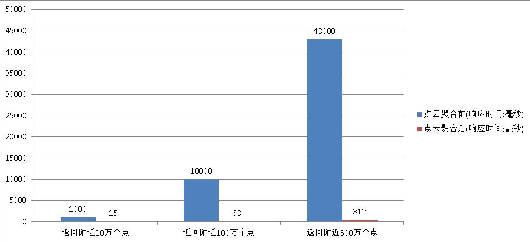
Performance comparison before and after aggregation
2 pgpointcloud
https://github.com/pgpointcloud/pointcloud

<LIDAR in PostgreSQL with PointCloud>
LIDAR sensors quickly produce millions of points with large numbers of variables measured on each point.

The challenge for a point cloud database extension is efficiently storing this data while allowing high fidelity access to the many variables stored.

Much of the complexity in handling LIDAR comes from the need to deal with multiple variables per point.

The variables captured by LIDAR sensors varies by sensor and capture process.

Some data sets might contain only X/Y/Z values.

Others will contain dozens of variables: X, Y, Z; intensity and return number; red, green, and blue values; return times; and many more.

There is no consistency in how variables are stored:
intensity might be stored in a 4-byte integer, or in a single byte; X/Y/Z might be doubles, or they might be scaled 4-byte integers.

PostgreSQL Pointcloud deals with all this variability by using a "schema document" to describe the contents of any particular LIDAR point.

Each point contains a number of dimensions, and each dimension can be of any data type,
with scaling and/or offsets applied to move between the actual value and the value stored in the database.

The schema document format used by PostgreSQL Pointcloud is the same one used by the PDAL library.
The pgpointcloud is a plug-in specifically designed to handle LIDAR data and is recommended.
3 LLVM(JIT)
PostgreSQL 10.0 preview Performance Enhancement - Launch of JIT Development Framework (Towards HTAP)
PostgreSQL Vectorization Execution Plug-in (Tile Implementation) 10x Speed Up OLAP
2. GiST index optimization
create index idx_cloudpoint_test_agg_1 on cloudpoint_test_agg using gist(loc_box) with (buffering=on);
create index idx_cloudpoint_test_1 on cloudpoint_test using gist(loc) with (buffering=on);
3. Streaming Return
Streaming returns have two methods, cursor and asynchronous message.
1. Cursors implement streaming returns.
begin;

declare cur1 cursor for select * from (select *, ST_Distance ( st_makepoint(5000,5000), loc ) as dist from cloudpoint_test order by st_makepoint(5000,5000) <-> loc ) t where dist < 1000;

fetch 100 from cur1;

fetch ...;

-- The client receives enough data, or when the distance exceeds, does not receive any more, closes the cursor, and exits the transaction.

close cur1;

end;
2. Streaming returns are achieved with asynchronous messages.
listen abcd;
Session 2, Initiate Request, Send Asynchronous Message to Listening Channel
create or replace function ff(geometry, float8, int, text) returns void as $$
declare
  v_rec record;
  v_limit int := $3;
begin
  set local enable_seqscan=off;   -- Forced Index, Scan lines enough to exit.
  for v_rec in
    select *,
    ST_Distance ( $1, loc ) as dist
    from cloudpoint_test
    order by loc <-> $1           -- Return from near to far in distance order
  loop
    if v_limit <=0 then           -- Determine if the number of records returned has reached LIMIT Number of records
      raise notice 'Sufficient limit Set % Bar data, But distance % Points within may also have.', $3, $2;
      return;
    end if;
    if v_rec.dist > $2 then       -- Determine if the distance is greater than the requested distance
      raise notice 'distance % Points within have been output', $2;
      return;
    else
      -- return next v_rec;
      perform pg_notify ($4, v_rec::text);
    end if;
    v_limit := v_limit -1;
  end loop;
end;
$$ language plpgsql strict volatile;
Session 2 initiates a search request
postgres=# select ff(st_makepoint(5000,5000), 1000, 10, 'abcd');
NOTICE:  Sufficient limit 10 sets of data, But points within 1,000 may still exist.
 ff
----

(1 row)
Session 1 will receive messages from channels asynchronously
Asynchronous notification "abcd" with payload "(38434407,01010000000060763E6E87B34000C0028CC587B340,test,0.613437682476958)" received from server process with PID 36946.
Asynchronous notification "abcd" with payload "(41792090,0101000000006008B91F88B3400000D5D13B87B340,test,0.776283650707887)" received from server process with PID 36946.
Asynchronous notification "abcd" with payload "(90599062,0101000000002057B2A888B34000C093516E88B340,test,0.787366330405518)" received from server process with PID 36946.
Asynchronous notification "abcd" with payload "(69482516,01010000000000A574AE88B34000601AEBA888B340,test,0.948568992176712)" received from server process with PID 36946.
Asynchronous notification "abcd" with payload "(12426846,0101000000006075D49188B34000E0E8E70487B340,test,1.13425697837729)" received from server process with PID 36946.
Asynchronous notification "abcd" with payload "(98299759,0101000000004054059388B340006014ED1089B340,test,1.21096126708341)" received from server process with PID 36946.
Asynchronous notification "abcd" with payload "(31175773,010100000000C03179EE88B34000A03E0C1B87B340,test,1.29136079279649)" received from server process with PID 36946.
Asynchronous notification "abcd" with payload "(11651191,01010000000080C6634C87B34000E0A4852689B340,test,1.34753214416354)" received from server process with PID 36946.
Asynchronous notification "abcd" with payload "(50248773,010100000000C064B3A686B34000809FA0F487B340,test,1.34955653568245)" received from server process with PID 36946.
Asynchronous notification "abcd" with payload "(28170573,010100000000608F958B86B34000C051C1F587B340,test,1.45529948415963)" received from server process with PID 36946.
4. HEAP discrete IO amplification optimization
8. Other applications of PostgreSQL in the field of GIS


Visual Mining and PostGIS Spatial Database Perfect Encounters - Advertising and Marketing Encounters
Chat about Technology-Logistics, Dynamic Route Planning Behind Double Eleven
9. Summary
PostgreSQL, PostGIS, pg-grid, pgpointcloud meet these three requirements very well.

10. Aliyun RDS PostgreSQL, the classic use of HybridDB PostgreSQL
RDS PostgreSQL
Responsible for OLTP and T+0 OLAP business, mainly in these areas
Huashan Lunjian tpc.org in the database field
PostgreSQL 10 has additional HTAP enhancements and will be launched in the near future.
Functionality is the strength of PostgreSQL, as detailed in PostgreSQL Past and Present.
Extended computing power, by adding CPU s, you can extend the performance of complex computing.
Cost of maintenance: With cloud services, the cost of operation and maintenance is almost zero.
HybridDB for PostgreSQL
Inherited from PostgreSQL, PostgreSQL is basically functionally close to PostgreSQL.
Cost of maintenance: With cloud services, the cost of operation and maintenance is almost zero.
Typical User Usage
Technology stack and cloud applications:

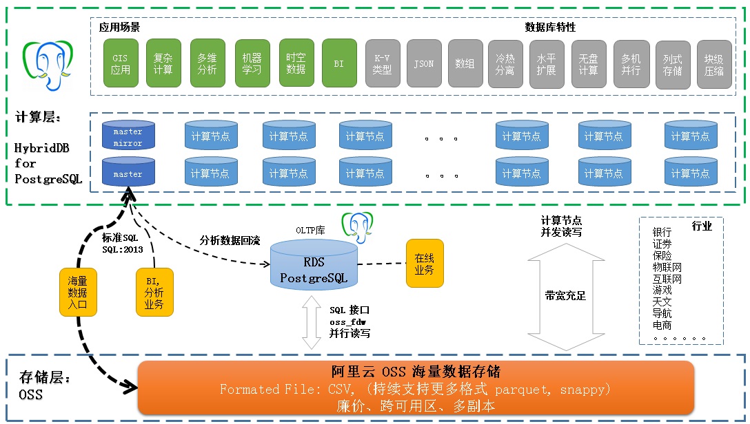
Separate cloud storage from computing usage:
RDS PostgreSQL: Read and Write OSS Object Storage Using oss_fdw
HybridDB PostgreSQL: Read and Write OSS Object Storage Using oss_fdw
11. Reference
http://s3.cleverelephant.ca/foss4gna2013-pointcloud.pdf
http://postgis.net/documentation/
Art and Technology Value of Honeycomb - PostgreSQL PostGIS's hex-grid
PostgreSQL Geographic Location Data Nearest Neighbor Query Performance
https://www.openstreetmap.org/#map=5/51.500/-0.100
https://www.postgresql.org/docs/9.6/static/sql-notify.html
https://www.postgresql.org/docs/9.6/static/libpq.html
http://postgis.net/docs/manual-2.3/ST_MakeBox2D.html