Task 1-1 linear regression notes

1, Explanation of linear regression model

1. What is a linear model

Representation data can be described by linetype relationship. In the case of formulation, y=wx+b. The process of modeling is the process of finding w, b.
However, due to the deviation of real data, unbiased estimation cannot be obtained, and only a model with the smallest deviation can be found.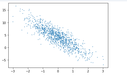

2. Solution of linear model

Basic concepts:
Dataset = training set + test set = sample + label
The sample is represented by characteristics (the characteristics related to house price include area, old and new, etc.)
The model hopes to establish the relationship between these characteristics and house price, so as to minimize the error between the predicted value and the real value, so that the predicted house price (predicted value) and the actual house price (real value) are closest

loss function

In model training, we need to measure the error between the predicted value and the real value. Generally, we choose a non negative number as the error, and the smaller the value is, the smaller the error is. A common choice is the square function. Its expression in evaluating the sample error with index iii is

l(i)(w,b)=12(y^(i)−y(i))2, l^{(i)}(\mathbf{w}, b) = \frac{1}{2} \left(\hat{y}^{(i)} - y^{(i)}\right)^2, l(i)(w,b)=21(y^(i)−y(i))2,

L(w,b)=1n∑i=1nl(i)(w,b)=1n∑i=1n12(w⊤x(i)+b−y(i))2. L(\mathbf{w}, b) =\frac{1}{n}\sum_{i=1}^n l^{(i)}(\mathbf{w}, b) =\frac{1}{n} \sum_{i=1}^n \frac{1}{2}\left(\mathbf{w}^\top \mathbf{x}^{(i)} + b - y^{(i)}\right)^2. L(w,b)=n1i=1∑nl(i)(w,b)=n1i=1∑n21(w⊤x(i)+b−y(i))2.

Optimization function

When the loss function can not be solved, it needs to be solved iteratively to approach the real value. In the optimization algorithm of numerical solution, mini batch stochastic gradient descent is widely used in deep learning. Its algorithm is very simple: first select the initial value of a group of model parameters, such as random selection; then iterate the parameters many times, so that each iteration may reduce the value of the loss function. In each iteration, a small batch (B \ match {B} b) consisting of a fixed number of training data samples is randomly and uniformly sampled, and then the derivative (gradient) of model parameters related to the average loss of data samples in small batch is calculated. Finally, the product of this result and a preset positive number is used as the reduction of model parameters in this iteration.

(w,b)←(w,b)−η∣B∣∑i∈B∂(w,b)l(i)(w,b) (\mathbf{w},b) \leftarrow (\mathbf{w},b) - \frac{\eta}{|\mathcal{B}|} \sum_{i \in \mathcal{B}} \partial_{(\mathbf{w},b)} l^{(i)}(\mathbf{w},b) (w,b)←(w,b)−∣B∣ηi∈B∑∂(w,b)l(i)(w,b)

Learning rate: η \ eta η represents the step size that can be learned in each optimization
Batch size: B \ batch {B} B is the batch size in small batch calculation

To summarize, there are two steps to optimize the function:

(i) Initialization of model parameters, generally using random initialization;
(ii) we iterate on the data several times, and update each parameter by moving the parameter in the negative gradient direction.

2, Explanation of linear regression code

1. Vector computing
Fast vector calculation
One way to add vectors is to add them scalar by element. c[i] = a[i] + b[i]
Another way to add vectors is to add these two vectors directly. d = a + b

2. Realization of linear regression model from zero

Header file

# import packages and modules
%matplotlib inline
import torch
from IPython import display
from matplotlib import pyplot as plt
import numpy as np
import random

print(torch.__version__)

Generate data

Suppose the model parameters w and b generate data, in order to make the data conform to the real situation, add fluctuations
Generate a data set of 1000 samples. The following is the linear relationship used to generate data:

price=warea⋅area+wage⋅age+b \mathrm{price} = w_{\mathrm{area}} \cdot \mathrm{area} + w_{\mathrm{age}} \cdot \mathrm{age} + b price=warea⋅area+wage⋅age+b

# set input feature number
num_inputs = 2
# set example number
num_examples = 1000

# set true weight and bias in order to generate corresponded label
true_w = [2, -3.4]
true_b = 4.2
#Generate 1000x2 random numbers as eigenvalues
features = torch.randn(num_examples, num_inputs,
                      dtype=torch.float32)
#According to the values of w and b, the corresponding labels of features are generated
labels = true_w[0] * features[:, 0] + true_w[1] * features[:, 1] + true_b
#Increase interference
labels += torch.tensor(np.random.normal(0, 0.01, size=labels.size()),
                       dtype=torch.float32)

Using images to show data

#Relationship between data feature [1] and label
plt.scatter(features[:, 1].numpy(), labels.numpy(), 1);

Read data

Divide data sets into small batches

#
def data_iter(batch_size, features, labels):
    num_examples = len(features)
    indices = list(range(num_examples))
    random.shuffle(indices)  # random read 10 samples
    for i in range(0, num_examples, batch_size):
        j = torch.LongTensor(indices[i: min(i + batch_size, num_examples)]) # the last time may be not enough for a whole batch
        yield  features.index_select(0, j), labels.index_select(0, j)

batch_size = 10

for X, y in data_iter(batch_size, features, labels):
    print(X, '\n', y)
    break

Procedure execution sequence:
for gets the iteratable object from the function data ITER and calls the next method.
Run data ITER to yield and return. Yield here is equivalent to return
After the value of for is given to X and y, proceed to the next iteration and continue the for loop in data item
Relevant knowledge:
generator : the function with yield is a generator (generator is a special kind of iterator), not a function. This generator has a function that is next function. Next is equivalent to the number generated in "next step". This time, the next start is executed in the place where next stops. So when next is called, the generator stops in the next step Stop at the beginning, and then return the number to be generated after meeting yield. This step is over.

The essence of the for item in iteratable loop is to obtain the iterator of iteratable object iteratable through the iter() function, and then call the next() method to get the next value and assign it to item. When encountering the exception of StopIteration, the loop ends.
reference:
Iterator() function and next() function for in... The essence of circulation
Understanding the for loop in Python : there are steps for the for loop to call the next method

Initialize model parameters

w = torch.tensor(np.random.normal(0, 0.01, (num_inputs, 1)), dtype=torch.float32)
b = torch.zeros(1, dtype=torch.float32)
#Set gradient properties
w.requires_grad_(requires_grad=True)
b.requires_grad_(requires_grad=True)

All the sensors have the. Requirements "grad property, which can be set. After that, you can call backward() to find the derivation.

Definition model

Define the training model for training parameters:
price=warea⋅area+wage⋅age+b \mathrm{price} = w_{\mathrm{area}} \cdot \mathrm{area} + w_{\mathrm{age}} \cdot \mathrm{age} + b price=warea⋅area+wage⋅age+b

def linreg(X, w, b):
    return torch.mm(X, w) + b

Define loss function

We use the mean square error loss function:
l(i)(w,b)=12(y^(i)−y(i))2, l^{(i)}(\mathbf{w}, b) = \frac{1}{2} \left(\hat{y}^{(i)} - y^{(i)}\right)^2, l(i)(w,b)=21(y^(i)−y(i))2,

def squared_loss(y_hat, y): 
    return (y_hat - y.view(y_hat.size())) ** 2 / 2

Define optimization function

Here, the optimization function uses random gradient descent of small batch:

  def sgd(params, lr, batch_size): 
    for param in params:
        param.data -= lr * param.grad / batch_size # ues .data to operate param without gradient track

train

When the data set, model, loss function and optimization function are defined, they can prepare for model training.

# super parameters init
lr = 0.03#Learning rate
num_epochs = 5#Training cycle

net = linreg
loss = squared_loss

# training
#Carry out 5 rounds of training, each round of training is solved in batches, and the accuracy of 5 rounds of results is averaged
for epoch in range(num_epochs):  # training repeats num_epochs times
    # in each epoch, all the samples in dataset will be used once
    
    # X is the feature and y is the label of a batch sample
    for X, y in data_iter(batch_size, features, labels):
        l = loss(net(X, w, b), y).sum()  
        # calculate the gradient of batch sample loss 
        l.backward()#Computational gradient  
        # Using small batch random gradient descent to item model parameters model solution
        sgd([w, b], lr, batch_size)  
        # reset parameter gradient
        w.grad.data.zero_()
        b.grad.data.zero_()
        #Model deviation
    train_l = loss(net(features, w, b), labels)
    print('epoch %d, loss %f' % (epoch + 1, train_l.mean().item()))

Automatic derivation Here l.backward() gets the derivative of loss for w and b, and x.grad gets the derivative

3. Simple implementation of pytorch

import torch
from torch import nn
import numpy as np
torch.manual_seed(1)

print(torch.__version__)
torch.set_default_tensor_type('torch.FloatTensor')

Generate data set

Generating datasets here is exactly the same as in a zero based implementation.

num_inputs = 2
num_examples = 1000

true_w = [2, -3.4]
true_b = 4.2

features = torch.tensor(np.random.normal(0, 1, (num_examples, num_inputs)), dtype=torch.float)
labels = true_w[0] * features[:, 0] + true_w[1] * features[:, 1] + true_b
labels += torch.tensor(np.random.normal(0, 0.01, size=labels.size()), dtype=torch.float)

Read data set

import torch.utils.data as Data

batch_size = 10

# combine featues and labels of dataset
dataset = Data.TensorDataset(features, labels)

# put dataset into DataLoader
data_iter = Data.DataLoader(
    dataset=dataset,            # torch TensorDataset format
    batch_size=batch_size,      # mini batch size
    shuffle=True,               # whether shuffle the data or not
    num_workers=2,              # read data in multithreading threads
)

for X, y in data_iter:
    print(X, '\n', y)
    break

Definition model

Define the class, network structure and propagation mode of line network

class LinearNet(nn.Module):
    def __init__(self, n_feature):
        super(LinearNet, self).__init__()      # call father function to init 
        self.linear = nn.Linear(n_feature, 1)  # function prototype: `torch.nn.Linear(in_features, out_features, bias=True)`

    def forward(self, x):
        y = self.linear(x)
        return y
    
net = LinearNet(num_inputs)
print(net)
LinearNet(
  (linear): Linear(in_features=2, out_features=1, bias=True)
)
# ways to init a multilayer network
# method one
net = nn.Sequential(
    nn.Linear(num_inputs, 1)
    # other layers can be added here
    )

# method two
net = nn.Sequential()
net.add_module('linear', nn.Linear(num_inputs, 1))
# net.add_module ......

# method three: put the neural network layer into the dictionary and pass it in
from collections import OrderedDict
net = nn.Sequential(OrderedDict([
          ('linear', nn.Linear(num_inputs, 1))
          # ......
        ]))

print(net)#All neural networks
print(net[0])#First floor

Initialize model parameters

Use init for initialization:

# 2. Normal distribution - N(mean, std)
# torch.nn.init.normal_(tensor, mean=0, std=1)
# 3. Constant - fixed value val
# torch.nn.init.constant_(tensor, val)
nn.init.constant_(w, 0.3)

from torch.nn import init

init.normal_(net[0].weight, mean=0.0, std=0.01)
init.constant_(net[0].bias, val=0.0)  # or you can use `net[0].bias.data.fill_(0)` to modify it directly

Define loss function

for param in net.parameters():
    print(param)
loss = nn.MSELoss()    # nn built-in squared loss function
                       # function prototype: `torch.nn.MSELoss(size_average=None, reduce=None, reduction='mean')

Define optimization function

import torch.optim as optim

optimizer = optim.SGD(net.parameters(), lr=0.03)   # Built in random gradient descent function
print(optimizer)  # function prototype: `torch.optim.SGD(params, lr=, momentum=0, dampening=0, weight_decay=0, nesterov=False)`

train

The two cycles, period and batch, y.view and reshape in numpy are the same, making the data arranged horizontally

num_epochs = 3
for epoch in range(1, num_epochs + 1):
    for X, y in data_iter:
        output = net(X)
        l = loss(output, y.view(-1, 1))
        optimizer.zero_grad() # reset gradient, equal to net.zero_grad()
        l.backward()#Back propagation calculation gradient
        optimizer.step()
    print('epoch %d, loss: %f' % (epoch, l.item()))#One output per cycle
# result comparision
dense = net[0]
print(true_w, dense.weight.data)
print(true_b, dense.bias.data)

A small ball

Published 23 original articles, won praise 3, visited 3820

Private letter follow

Posted by Tr4mpldUndrfooT on Thu, 13 Feb 2020 04:31:10 -0800

Programmer Group

Task 1-1 linear regression notes

1, Explanation of linear regression model

1. What is a linear model

2. Solution of linear model

loss function

Optimization function

2, Explanation of linear regression code

2. Realization of linear regression model from zero

Header file

Generate data

Read data

Initialize model parameters

Definition model

Define loss function

Define optimization function

train

3. Simple implementation of pytorch

Generate data set

Read data set

Definition model

Initialize model parameters

Define loss function

Define optimization function

train

Hot Keywords