Survival analysis involves the prediction of the time of a particular event. It is also called failure time analysis or analysis of death time.

For example, we can predict the survival days of cancer patients or the failure time of mechanical system.

The software package survival in R is used for survival analysis. The package contains the Surv() function, which takes the input data as the R formula, creates a survival object in the selected variable for analysis, and then uses the survfit() function to create the analysis diagram. The syntax is as follows:

Surv(time,event)
survfit(formula)

The parameters are described as follows:

• Time - is the time until the event occurs.
• Event - indicates the status of the expected event.
• formula - is the relationship between forecast variables.

Next, we use the data set named "pbc" existing in the installed survival package, which describes the survival data of patients with primary biliary cirrhosis (PBC).

In many of the columns that exist in the dataset, we focus on the "time" and "status" fields, where time represents the number of days before patients and events are registered between patients undergoing liver transplantation or dying patients. Let's look at the initial data:

setwd("D:/r_file")
# Load the library.
library("survival")

# Print first few rows.
print(head(pbc))

The output result is:

  id time status trt      age sex ascites hepato spiders edema bili chol
1  1  400      2   1 58.76523   f       1      1       1   1.0 14.5  261
2  2 4500      0   1 56.44627   f       0      1       1   0.0  1.1  302
3  3 1012      2   1 70.07255   m       0      0       0   0.5  1.4  176
4  4 1925      2   1 54.74059   f       0      1       1   0.5  1.8  244
5  5 1504      1   2 38.10541   f       0      1       1   0.0  3.4  279
6  6 2503      2   2 66.25873   f       0      1       0   0.0  0.8  248
  albumin copper alk.phos    ast trig platelet protime stage
1    2.60    156   1718.0 137.95  172      190    12.2     4
2    4.14     54   7394.8 113.52   88      221    10.6     3
3    3.48    210    516.0  96.10   55      151    12.0     4
4    2.54     64   6121.8  60.63   92      183    10.3     4
5    3.53    143    671.0 113.15   72      136    10.9     3
6    3.98     50    944.0  93.00   63       NA    11.0     3

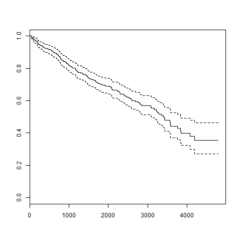
Let's continue to apply the Surv() function to the above datasets and create a trend graph that will display as follows:

setwd("D:/r_file")
# Load the library.
library("survival")

# Create the survival object. 
survfit(Surv(pbc$time,pbc$status == 2)~1)

# Give the chart file a name.
png(file = "survival.png")

# Plot the graph. 
plot(survfit(Surv(pbc$time,pbc$status == 2)~1))

# Save the file.
dev.off()

The output data is as follows:

Call: survfit(formula = Surv(pbc$time, pbc$status == 2) ~ 1)

      n  events  median 0.95LCL 0.95UCL 
    418     161    3395    3090    3853

The resulting image is as follows:

Well, that's the record.

If you feel good, please support me...