Article directory
Data exploration
The original data download address is: Portal
The website describes the data as follows:
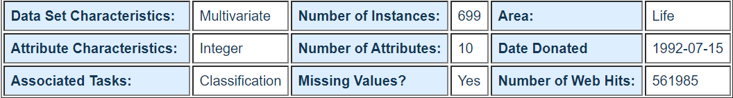
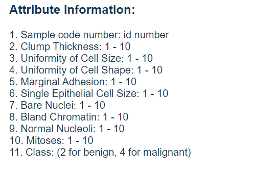
It can be seen that there are 699 samples in the original data, each sample has 11 different columns of values: 1 column of ID for retrieval, 9 columns of medical characteristics related to tumor, and the last column of values representing tumor type. All the 9 columns used to represent the medical characteristics of tumors were quantified as numbers between 1 and 10, and the types of tumors were also referred to as benign and malignant by the numbers 2 and 4 respectively. This data also states that it contains missing values. In fact, the problem of missing values widely exists in real data, which is also an unavoidable problem for machine learning tasks.
Data preprocessing
The following code is used to preprocess the original tumor data:
#Import pandas and numpy toolkits.
import pandas as pd
import numpy as np
#Create a feature list.
column_names = ['Sample code number', 'Clump Thickness',
                'Uniformity of Cell Size', 'Uniformity of Cell Shape',
                'Marginal Adhesion','Single Epithelial CellSize',
                'Bare Nuclei', 'Bland Chromatin', 'Normal Nucleoli',
                'Mitoses', 'Class']
#Use the pandas.readcsv function to read the specified data from the Internet.
data = pd.read_csv('breast-cancer-wisconsin.data', names=column_names)
#Replace? With the standard missing value.
data = data.replace (to_replace='?',value= np.nan)
#Discard data with missing values (as long as one dimension is missing).
data = data.dropna(how='any')
#Output data volume and dimension.
data.shape
(683, 11)
After data processing, there are 683 samples without missing values, including 9 dimensions, such as cell thickness, cell size, shape, etc., and the characteristics of each dimension are quantified as values between 1 and 10.
print(data.head())
   Sample code number  Clump Thickness  Uniformity of Cell Size  \
0             1000025                5                        1
1             1002945                5                        4
2             1015425                3                        1
3             1016277                6                        8
4             1017023                4                        1

   Uniformity of Cell Shape  Marginal Adhesion  Single Epithelial CellSize  \
0                         1                  1                           2
1                         4                  5                           7
2                         1                  1                           2
3                         8                  1                           3
4                         1                  3                           2

  Bare Nuclei  Bland Chromatin  Normal Nucleoli  Mitoses  Class
0           1                3                1        1      2
1          10                3                2        1      2
2           2                3                1        1      2
3           4                3                7        1      2
4           1                3                1        1      2
Since the original data does not provide the corresponding test samples to evaluate the model performance, it is necessary to
The data is divided. 15% of the data will be used as the test set, and the remaining 75% will be used for training.
#Use the train test split module in sklearn.cross-validation to split the data.
from sklearn.cross_validation import train_test_split
#Random sampling 25% of the data for testing, the remaining 75% for building training sets.
x_train, x_test, y_train,y_test = train_test_split (data [column_names[1:10]],
                                                    data [column_names[10]],
                                                    test_size=0.25, random_state= 33)
#Check the number and category distribution of training samples.
y_train.value_counts()
2    344
4    168
Name: Class, dtype: int64
#Check the number and category distribution of test samples.
y_test.value_counts()
2    100
4     71
Name: Class, dtype: int64
To sum up, we used 512 training samples (344 benign tumor data, 168 malignant tumor data) to test
There were 171 samples (100 benign tumor data, 71 malignant tumor data).
model building
Next, we use Logistic regression and random gradient parameter estimation
Methods the training data after the above processing were studied and predicted according to the characteristics of test samples.
 #Guide StandardScaler from sklearn.preprocessing
from sklearn. preprocessing import StandardScaler
#From the sklearn. Linear? Model, guide LogisticRegression and SGDClassifier
from sklearn. linear_model import LogisticRegression
from sklearn.linear_model import SGDClassifier
#Standardize the data to ensure that the variance of each dimension's characteristic data is 1 and the mean value is 0. So that the prediction results will not be dominated by some dimension too large eigenvalues.
ss = StandardScaler ()
x_train = ss.fit_transform(x_train)
x_test = ss.transform(x_test)
#Initialize logisticrenewal and SGDClassifier
lr = LogisticRegression ()
sgdc = SGDClassifier ()
#Call the fit function in LogisticRegression to train model parameters.
lr.fit(x_train, y_train)
#The trained model LR is used to predict the x'u test, and the results are stored in the variable lr'y predict.
lr_y_predict = lr.predict(x_test)
#Call the fit function in SGDClassifier to train the model parameters.
sgdc.fit (x_train, y_train)
#The trained model sgdc is used to predict the X ﹣ test, and the results are stored in the variable sgdc ﹣ y ﹣ predict.
sgdc_y_predict = sgdc.predict(x_test)
C:\ProgramData\Anaconda3\lib\site-packages\sklearn\linear_model\stochastic_gradient.py:128: FutureWarning: max_iter and tol parameters have been added in <class 'sklearn.linear_model.stochastic_gradient.SGDClassifier'> in 0.19. If both are left unset, they default to max_iter=5 and tol=None. If tol is not None, max_iter defaults to max_iter=1000. From 0.21, default max_iter will be 1000, and default tol will be 1e-3.
  "and default tol will be 1e-3." % type(self), FutureWarning)
Display of forecast results
Using logistic regression and SGDClassifier to predict 171 test samples respectively. Because these 171 test samples have correct marks and are recorded in the variable y_test, it is very intuitive to compare the predicted results with the original correct marks and calculate the correct percentage of the 171 test samples, that is, the correct rate.
#Guide the classification report module from sklearn. Metrics.
from sklearn.metrics import classification_report
#Use the score function of Logistic regression model to get the accuracy of the model on the test set.
print('Accuracy of LR Classifier:', lr.score(x_test, y_test))
#The classification report module is used to get the results of the other three indicators of LogisticRegression.
print(classification_report(y_test, lr_y_predict, target_names = ['Benign','Malignant']))
Accuracy of LR Classifier: 0.9883040935672515
             precision    recall  f1-score   support

     Benign       0.99      0.99      0.99       100
  Malignant       0.99      0.99      0.99        71

avg / total       0.99      0.99      0.99       171
#The score function of the random gradient descent model is used to get the accuracy of the model on the test set.
print ('Accuarcy of SGD Classifier:', sgdc.score(x_test, y_test))
 #The other three indexes of SGDClassifier are obtained by using the classification report module.
print (classification_report(y_test, sgdc_y_predict, target_names= [' Benign','Malignant']))
Accuarcy of SGD Classifier: 0.9824561403508771
             precision    recall  f1-score   support

     Benign       0.98      0.99      0.99       100
  Malignant       0.99      0.97      0.98        71

avg / total       0.98      0.98      0.98       171
conclusion
After reading the code 16 output report, we can find that: logistic regression has a higher accuracy in test set performance than SGDClassifier. This is because seikit learn uses analytic method to calculate the parameters of LogisticRegression accurately, and uses gradient method to estimate the parameters of SGDClassifier.

