catalogue
2. Pseudolabel method for deep neural networks
3. Why could Pseudo-Label work? (why pseudo tags work)
3.1. Low density separation between classes
3.3. Training with pseudo label as entropy regularization
4.1. Handwritten digital recognition (MNIST)
2. Mean Teacher (average teacher)
3.1 Comparison to other methods on SVHN and CIFAR-10
3.2 SVHN with extra unlabeled data
3.3 Analysis of the training curves
Deep labv3 + network code implementation
Plans completed this week
- Read the paper pseudolabel: the simple and efficient semi supervised learning method for deep neural networks
- Read the paper mean teachers: weight averaged consistency targets improve semi supervised
- Running model: DeepLabv3 +, Deeplab series networks were proposed by Geogle. After V2, atrus spatial pyramid pooling (ASPP) was mainly introduced to fuse multi-scale information by hole convolution with different expansion factors. In fact, hole convolution (convolution with holes) is used to operate image features with different rates.
Thesis Reading 1
Pseudolabel: the simple and efficient semi supervised learning method for deep neural networks
Abstract (Abstract)
A simple and effective semi supervised learning method of deep neural network is proposed. Basically, the proposed network is trained by using labeled and unlabeled data simultaneously in a supervised way. For unlabeled data, pseudo labels can be used only by selecting the category with the greatest prediction probability , as if they were true labels. This is actually equivalent to Entropy Regularization. It supports low-density separation between classes On MNIST handwritten numeral data set, using denoising automatic encoder and Dropout, this simple method is better than the traditional semi supervised learning method when there are very few label data.
1. Introduction
In this paper, we propose a simpler method to train neural networks in a semi supervised way. For unlabeled data, we only need to select the class with the maximum prediction probability for each weight update, and we can use pseudo labels as if they were true labels. In principle, this method can combine almost all neural network models and training methods. This method is practical It is equivalent to entropy regularization. The conditional entropy of class probability can be used to measure class overlap. By minimizing the entropy of unlabeled data, the overlap of class probability distribution can be reduced. It supports low-density separation between classes, which is a priori condition commonly assumed by semi supervised learning.
Experiments on the famous MNIST dataset show that this method has the best state of the art performance.
2. Pseudolabel method for deep neural networks
2.1. Deep Neural Networks
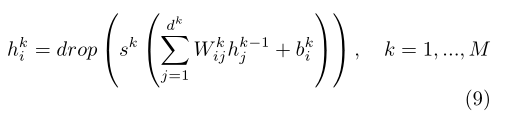
Pseudo tagging is a semi supervised method for training deep neural networks. In this paper, we will consider multilayer neural networks with M-layer hidden units:
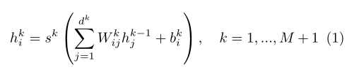
 Is the nonlinear activation function of layer k, such as Sigmoid. The whole network can be trained by minimizing the supervised loss function.
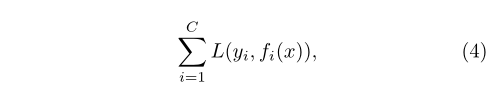
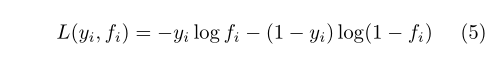
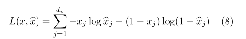
Where C is the number of tags and x is the input vector. We can choose cross entropy as the loss function:
2.2. Denoising auto encoder
Denoising self coder is an unsupervised learning algorithm, which is based on the idea that the learned representations are robust to even partially damaged inputs (Vincent et al., 2008). This method can be used to train automatic coders and stack these DAE s to initialize deep neural networks.
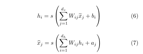
 Is the j-th part of the corrupted input value,
 Is the reconstruction of the j-th input value. The training of automatic encoder is to minimize theandReconstruction error between. For binary input values, the common choice of reconstruction error is cross entropy:
We used DAE in the unsupervised pre training stage with a probability of 0.5 for masking noise corruption.
2.3. Dropout
Dropout is a supervised learning technique that can be applied to deep neural networks (Hinton et al., 2012). On the network activation of each example, the hidden units are omitted (inactivated) randomly with a probability of 0.5. Sometimes, 20% of the visible units are lost.
This technique can reduce over fitting to prevent complex co adaptations to the hidden representation of training data, because in each weight update, we train different sub models by omitting half of the hidden units.
2.4. Pseudo label
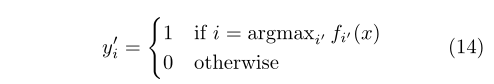
Pseudo label target classes of unlabeled data as if they were real labels. We only select the category with the greatest prediction probability for each unlabeled sample.
Labeled data and unlabeled data train the pre trained network in a supervised manner at the same time . for unlabeled data, the recalculated pseudo tags for each weight update are used for the loss function of the same supervised learning task. Since the total number of labeled data and unlabeled data is very different, and the training balance between them is very important to network performance, the overall loss function is:
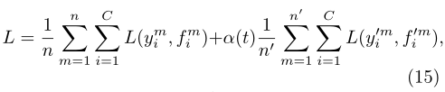
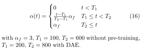
N is the number of small batches with labeled data, n 'is unlabeled data, ymi is the label with labeled data, fmi is the predicted value of the model with labeled data, y'mi is the pseudo label, and f'mi is the predicted value of the unlabeled data model, α (t) Is the coefficient that balances them.
α (t) Reasonable scheduling is very important to network performance. If α (t) Too high will interfere with training even for marked data. And if α (t) Too small, we cannot take advantage of unlabeled data. In addition, α (t) The slowly increasing deterministic annealing process is expected to help the optimization process avoid poor local minima, so that the pseudo tags of unlabeled data are similar to the real tags as much as possible.
3. Why could Pseudo-Label work? (why pseudo tags work)
3.1. Low density separation between classes
The goal of semi supervised learning is to improve generalization performance using unlabeled data ). The clustering hypothesis points out that the decision boundary should be located in the low-density region to improve the generalization performance. Semi supervised embedding (Weston et al., 2008) uses embedding based regularization to improve the generalization performance of deep neural networks. Because the neighborhood of data samples has similar activation with the samples through embedding penalty terms, the data samples in the high-density region are more likely to have the same label.
3.2. Entropy Regularization
Entropy regularization (Grandvalet et al., 2006) is a method that benefits from unlabeled data under the framework of maximum a posteriori estimation. This scheme supports low-density separation between classes by minimizing the conditional entropy of class probability of unlabeled data without any density modeling.
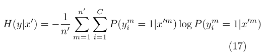
Entropy is a measure of class overlap. With the reduction of class overlap, the density of data points on the decision boundary becomes lower.
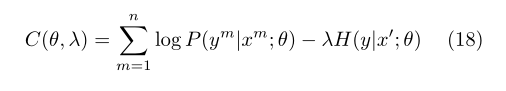
By maximizing the conditional log likelihood of labeled data (item 1) and minimizing the entropy of unlabeled data (item 2), better generalization performance can be obtained by using unlabeled data.
3.3. Training with pseudo label as entropy regularization
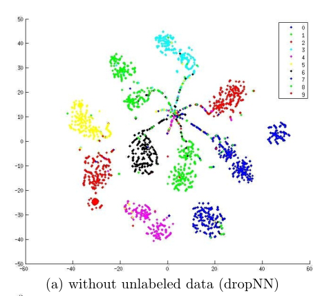
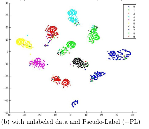
Fig. 1 shows MNIST test data for t-SNE dimensionality reduction (not included in unlabeled data) The neural network is trained with 600 labeled data, with or without 60000 unlabeled data and pseudo tags. Although the training error is zero in both cases, by using unlabeled data and pseudo tags for training, the network output of test data is more concentrated near 1 of K code, in other words, entropy is minimized.
4. Experiments
4.1. Handwritten digital recognition (MNIST)
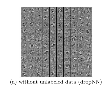
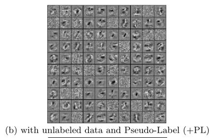
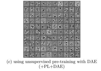
It can be seen that adding pseudo tags and denoising self encoder is the best effect of restoration.
5. Conclusion
In this work, we show a simple and effective neural network semi supervised learning method, which has the best performance without complex training scheme and high computational cost similarity matrix.
Thesis Reading 2
Mean teachers are better role models: weight averaged consistency targets improve semi supervised deep learning results
Abstract (Abstract)
The recently proposed temporal embedding model has achieved the most advanced results in several semi supervised learning benchmarks. It maintains the exponential moving average of the label prediction of each training sample and punishes the prediction inconsistent with the target. However, because the target changes only once in each Epoch, temporal embedding becomes very clumsy when learning large data sets. In order to overcome the problem To solve this problem, we propose the Mean Teacher model, a method of average model weight rather than label prediction. As an additional benefit, Mean Teacher improves the accuracy of testing and can use fewer labels for training than temporary embedding.
1. Introduction
Deep learning has achieved great success in the fields of image and speech recognition In addition, it is usually expensive to manually add high-quality labels to training data. Therefore, in semi supervised learning, regularization method needs to be used to effectively use unlabeled data to reduce over fitting.
There are at least two ways to improve the quality of the target. One is to carefully select the disturbance of the representation, rather than just applying additive or multiplicative noise. The other is to carefully select the teacher model, rather than reluctantly copy the student model. Therefore, our goal is to form a better teacher model from the student model without additional training.
2. Mean Teacher (average teacher)
In order to overcome the limitations of temporary embedding, we propose the average model weight instead of prediction. Since the teacher model is the average value of continuous student model, we call it the average teacher method (Fig. 2).
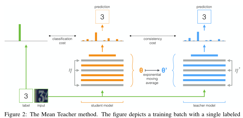
Figure 2: average teacher method. This figure describes a training batch with a single label sample. Both the student model and the teacher model evaluate the application noise within their calculation range( η,η 0). Use classification cost ) Compare the Softmax output of the student model with the one hot label and compare it with the teacher output using the consistency cost. After updating the weight of the student model with the gradient descent, the weight of the teacher model is updated to the exponential moving average of the student weight. The output of both models can be used for prediction, but the teacher's prediction is more likely at the end of the training Yes. The training steps with unlabeled samples will be similar, but classification cost will not be applied ).
The teacher model uses the EMA weights of the student model rather than sharing the weights with the student model. Now it can collect information at every step rather than after every era. In addition, the target model has a better intermediate representation because the weight average improves the output of all layers, not just the top output. These aspects lead to better intermediate representation than the temporary embedding model Two practical advantages: first, more accurate target labels lead to faster feedback loops between student and teacher models, resulting in better test accuracy. Second, the method is suitable for large data sets and online learning.
More formally, we define consistency cost as the expected distance between the prediction of student model and that of teacher model.

Π The difference between model, temporary embedding and average teacher lies in how teacher prediction is generated, Π Model use θ'=θ, Temporal embedding uses the weighted average of continuous predictions to approximate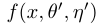 , we will
 Defined as when the training step is t, continuous θ The EMA value of the weight.

3. Experiments
To test our hypothesis, we first copied it in TensorFlow Π Model as baseline. Then, we modified the baseline model to use the weighted average consistency goal. The structure of the model is a 13 layer convolutional neural network (ConvNet), which has three types of noise: random translation and horizontal flip of the input image, Gaussian noise on the input layer and Dropout noise applied in the network.
3.1 Comparison to other methods on SVHN and CIFAR-10
We conducted experiments using street view house numbers and CIFAR-10 benchmarks. Both data sets contain 32x32 pixel RGB images belonging to ten different categories.
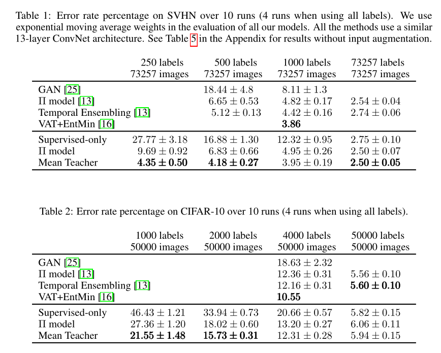
Tables 1 and 2 compare the results with recent state-of-the-art methods. All methods in the comparison use a similar 13 layer ConvNet architecture. Compared to Π Model and temporary embedding our Mean Teacher improves the test accuracy on semi supervised SVHN tasks. Mean Teacher also improved the performance of CIFAR-10, exceeding our baseline Π Model.
The recently published version of Virtual Adversarial Training by Miyato et al. Performs even better than Mean Teacher on 1000 label SVHN and 4000 label CIFAR-10. As discussed in the introduction, VAT and Mean Teacher are complementary approaches. Their combination may produce better accuracy than using any of them alone, but this research is beyond the scope of this article.
3.2 SVHN with extra unlabeled data
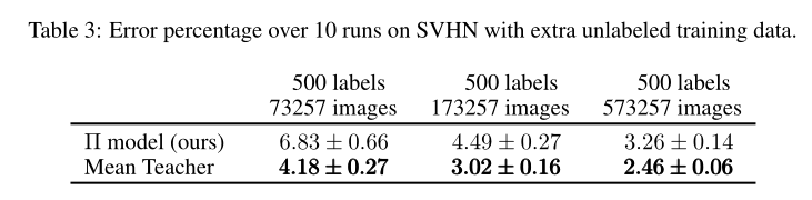
As mentioned above, our proposed Mean Teacher model can well adapt to large data sets and online learning. The experimental results of SVHN and CIFAR-10 show that the algorithm makes effective use of unlabeled samples. Therefore, we want to test whether we have reached the limit of our method. Table 3 shows the results:
3.3 Analysis of the training curves
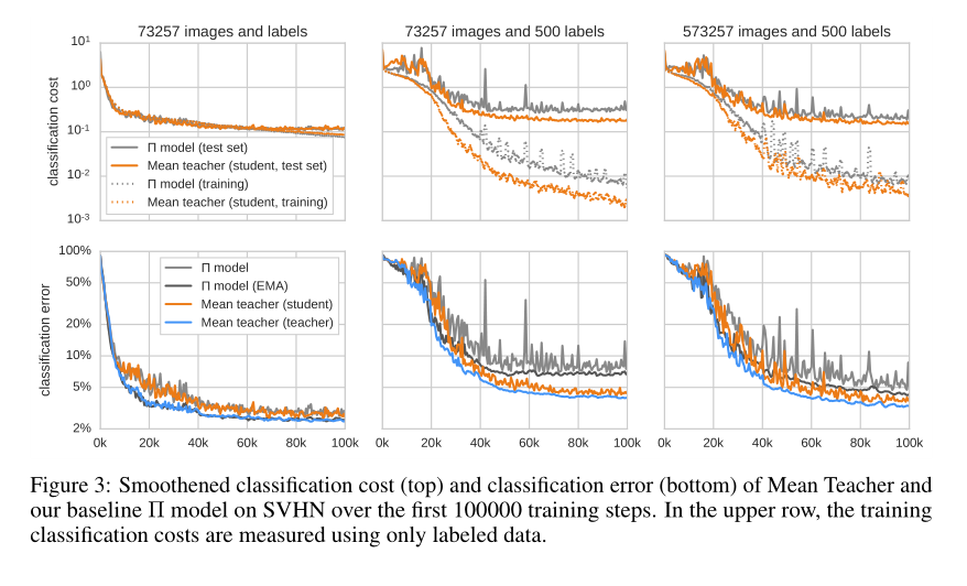
Figure 3: average teacher classification cost after smoothing ) (top) and classification error (bottom), and our baseline based on SVHN in the first 100000 training steps Π Model.
It can be seen from the figure that teachers (blue curve) improve students (Orange) through consistency cost and students improve teachers through exponential moving averaging, which seems to be a benign feedback cycle. If you leave this feedback cycle, the learning speed will slow down and the model will start over fitting earlier (dark gray and light gray).
4.Conclusion
In this paper, we propose Mean Teacher, a method of averaging model weight to form a goal generating teacher model. Different from temporary embedding, Mean Teacher uses large data sets and online learning. Experiments show that the algorithm improves the learning speed and classification accuracy of the training network. In addition, it can be well extended to the most advanced framework Structure and large image size.
Deep labv3 + network code implementation
import os, cv2
import numpy as np
import pandas as pd
import random, tqdm
import seaborn as sns
import matplotlib.pyplot as plt
%matplotlib inline
import warnings
warnings.filterwarnings("ignore")
import torch
import torch.nn as nn
from torch.utils.data import DataLoader
import albumentations as album
# !pip install -q -U segmentation-models-pytorch albumentations > /dev/null
import segmentation_models_pytorch as smp
# Defining train / val / test directories
DATA_DIR = '../input/massachusetts-buildings-dataset/tiff/'
x_train_dir = os.path.join(DATA_DIR, 'train')
y_train_dir = os.path.join(DATA_DIR, 'train_labels')
x_valid_dir = os.path.join(DATA_DIR, 'val')
y_valid_dir = os.path.join(DATA_DIR, 'val_labels')
x_test_dir = os.path.join(DATA_DIR, 'test')
y_test_dir = os.path.join(DATA_DIR, 'test_labels')
class_dict = pd.read_csv("../input/massachusetts-buildings-dataset/label_class_dict.csv")
# Get class names
class_names = class_dict['name'].tolist()
# Get class RGB values
class_rgb_values = class_dict[['r','g','b']].values.tolist()
print('All dataset classes and their corresponding RGB values in labels:')
print('Class Names: ', class_names)
print('Class RGB values: ', class_rgb_values)
# Shortlist specific classes to segment
# Useful to shortlist specific classes in datasets with large number of classes
select_classes = ['background', 'building']
# Get RGB values of required classes
select_class_indices = [class_names.index(cls.lower()) for cls in select_classes]
select_class_rgb_values = np.array(class_rgb_values)[select_class_indices]
print('Selected classes and their corresponding RGB values in labels:')
print('Class Names: ', class_names)
print('Class RGB values: ', class_rgb_values)
# Helper functions for viz. & one-hot encoding/decoding
# helper function for data visualization
def visualize(**images):
"""
Plot images in one row
"""
n_images = len(images)
plt.figure(figsize=(20,8))
for idx, (name, image) in enumerate(images.items()):
plt.subplot(1, n_images, idx + 1)
plt.xticks([]);
plt.yticks([])
# get title from the parameter names
plt.title(name.replace('_',' ').title(), fontsize=20)
plt.imshow(image)
plt.show()
# Perform one hot encoding on label
def one_hot_encode(label, label_values):
"""
Convert a segmentation image label array to one-hot format
by replacing each pixel value with a vector of length num_classes
# Arguments
label: The 2D array segmentation image label
label_values
# Returns
A 2D array with the same width and hieght as the input, but
with a depth size of num_classes
"""
semantic_map = []
for colour in label_values:
equality = np.equal(label, colour)
class_map = np.all(equality, axis = -1)
semantic_map.append(class_map)
semantic_map = np.stack(semantic_map, axis=-1)
return semantic_map
# Perform reverse one-hot-encoding on labels / preds
def reverse_one_hot(image):
"""
Transform a 2D array in one-hot format (depth is num_classes),
to a 2D array with only 1 channel, where each pixel value is
the classified class key.
# Arguments
image: The one-hot format image
# Returns
A 2D array with the same width and hieght as the input, but
with a depth size of 1, where each pixel value is the classified
class key.
"""
x = np.argmax(image, axis = -1)
return x
# Perform colour coding on the reverse-one-hot outputs
def colour_code_segmentation(image, label_values):
"""
Given a 1-channel array of class keys, colour code the segmentation results.
# Arguments
image: single channel array where each value represents the class key.
label_values
# Returns
Colour coded image for segmentation visualization
"""
colour_codes = np.array(label_values)
x = colour_codes[image.astype(int)]
return x
class BuildingsDataset(torch.utils.data.Dataset):
"""Massachusetts Buildings Dataset. Read images, apply augmentation and preprocessing transformations.
Args:
images_dir (str): path to images folder
masks_dir (str): path to segmentation masks folder
class_rgb_values (list): RGB values of select classes to extract from segmentation mask
augmentation (albumentations.Compose): data transfromation pipeline
(e.g. flip, scale, etc.)
preprocessing (albumentations.Compose): data preprocessing
(e.g. noralization, shape manipulation, etc.)
"""
def __init__(
self,
images_dir,
masks_dir,
class_rgb_values=None,
augmentation=None,
preprocessing=None,
):
self.image_paths = [os.path.join(images_dir, image_id) for image_id in sorted(os.listdir(images_dir))]
self.mask_paths = [os.path.join(masks_dir, image_id) for image_id in sorted(os.listdir(masks_dir))]
self.class_rgb_values = class_rgb_values
self.augmentation = augmentation
self.preprocessing = preprocessing
def __getitem__(self, i):
# read images and masks
image = cv2.cvtColor(cv2.imread(self.image_paths[i]), cv2.COLOR_BGR2RGB)
mask = cv2.cvtColor(cv2.imread(self.mask_paths[i]), cv2.COLOR_BGR2RGB)
# one-hot-encode the mask
mask = one_hot_encode(mask, self.class_rgb_values).astype('float')
# apply augmentations
if self.augmentation:
sample = self.augmentation(image=image, mask=mask)
image, mask = sample['image'], sample['mask']
# apply preprocessing
if self.preprocessing:
sample = self.preprocessing(image=image, mask=mask)
image, mask = sample['image'], sample['mask']
return image, mask
def __len__(self):
# return length of
return len(self.image_paths)
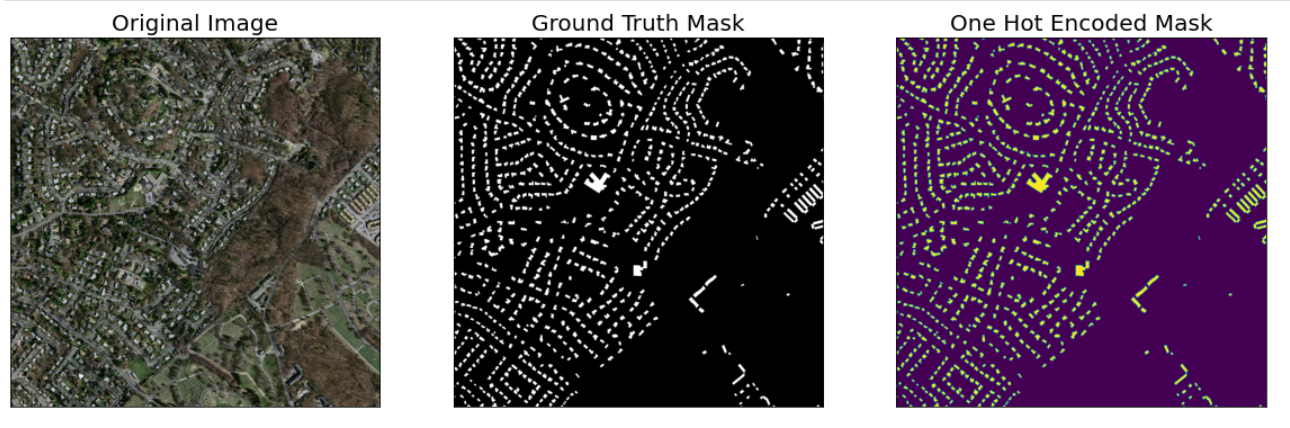
# Visualize Sample Image and Mask
dataset = BuildingsDataset(x_train_dir, y_train_dir, class_rgb_values=select_class_rgb_values)
random_idx = random.randint(0, len(dataset)-1)
image, mask = dataset[2]
visualize(
original_image = image,
ground_truth_mask = colour_code_segmentation(reverse_one_hot(mask), select_class_rgb_values),
one_hot_encoded_mask = reverse_one_hot(mask)
)
# Defining Augmentations
def get_training_augmentation():
train_transform = [
album.RandomCrop(height=256, width=256, always_apply=True),
album.OneOf(
[
album.HorizontalFlip(p=1),
album.VerticalFlip(p=1),
album.RandomRotate90(p=1),
],
p=0.75,
),
]
return album.Compose(train_transform)
def get_validation_augmentation():
# Add sufficient padding to ensure image is divisible by 32
test_transform = [
album.PadIfNeeded(min_height=1536, min_width=1536, always_apply=True, border_mode=0),
]
return album.Compose(test_transform)
def to_tensor(x, **kwargs):
return x.transpose(2, 0, 1).astype('float32')
def get_preprocessing(preprocessing_fn=None):
"""Construct preprocessing transform
Args:
preprocessing_fn (callable): data normalization function
(can be specific for each pretrained neural network)
Return:
transform: albumentations.Compose
"""
_transform = []
if preprocessing_fn:
_transform.append(album.Lambda(image=preprocessing_fn))
_transform.append(album.Lambda(image=to_tensor, mask=to_tensor))
return album.Compose(_transform)
# Visualize Augmented Images & Masks
augmented_dataset = BuildingsDataset(
x_train_dir, y_train_dir,
augmentation=get_training_augmentation(),
class_rgb_values=select_class_rgb_values,
)
random_idx = random.randint(0, len(augmented_dataset)-1)
# Different augmentations on a random image/mask pair (256*256 crop)
for i in range(3):
image, mask = augmented_dataset[random_idx]
visualize(
original_image = image,
ground_truth_mask = colour_code_segmentation(reverse_one_hot(mask), select_class_rgb_values),
one_hot_encoded_mask = reverse_one_hot(mask)
)
# Model Definition
ENCODER = 'resnet101'
ENCODER_WEIGHTS = 'imagenet'
CLASSES = class_names
ACTIVATION = 'sigmoid' # could be None for logits or 'softmax2d' for multiclass segmentation
# create segmentation model with pretrained encoder
model = smp.DeepLabV3Plus(
encoder_name=ENCODER,
encoder_weights=ENCODER_WEIGHTS,
classes=len(CLASSES),
activation=ACTIVATION,
)
preprocessing_fn = smp.encoders.get_preprocessing_fn(ENCODER, ENCODER_WEIGHTS)
# Get train and val dataset instances
train_dataset = BuildingsDataset(
x_train_dir, y_train_dir,
augmentation=get_training_augmentation(),
preprocessing=get_preprocessing(preprocessing_fn),
class_rgb_values=select_class_rgb_values,
)
valid_dataset = BuildingsDataset(
x_valid_dir, y_valid_dir,
augmentation=get_validation_augmentation(),
preprocessing=get_preprocessing(preprocessing_fn),
class_rgb_values=select_class_rgb_values,
)
# Get train and val data loaders
train_loader = DataLoader(train_dataset, batch_size=16, shuffle=True, num_workers=5)
valid_loader = DataLoader(valid_dataset, batch_size=1, shuffle=False, num_workers=2)
# Set Hyperparams
# Set flag to train the model or not. If set to 'False', only prediction is performed (using an older model checkpoint)
TRAINING = True
# Set num of epochs
EPOCHS = 80
# Set device: `cuda` or `cpu`
DEVICE = torch.device("cuda" if torch.cuda.is_available() else "cpu")
# define loss function
loss = smp.utils.losses.DiceLoss()
# define metrics
metrics = [
smp.utils.metrics.IoU(threshold=0.5),
]
# define optimizer
optimizer = torch.optim.Adam([
dict(params=model.parameters(), lr=0.0001),
])
# define learning rate scheduler (not used in this NB)
lr_scheduler = torch.optim.lr_scheduler.CosineAnnealingWarmRestarts(
optimizer, T_0=1, T_mult=2, eta_min=5e-5,
)
# load best saved model checkpoint from previous commit (if present)
if os.path.exists('../input/deeplabv3-efficientnetb4-frontend-using-pytorch/best_model.pth'):
model = torch.load('../input/deeplabv3-efficientnetb4-frontend-using-pytorch/best_model.pth', map_location=DEVICE)
train_epoch = smp.utils.train.TrainEpoch(
model,
loss=loss,
metrics=metrics,
optimizer=optimizer,
device=DEVICE,
verbose=True,
)
valid_epoch = smp.utils.train.ValidEpoch(
model,
loss=loss,
metrics=metrics,
device=DEVICE,
verbose=True,
)
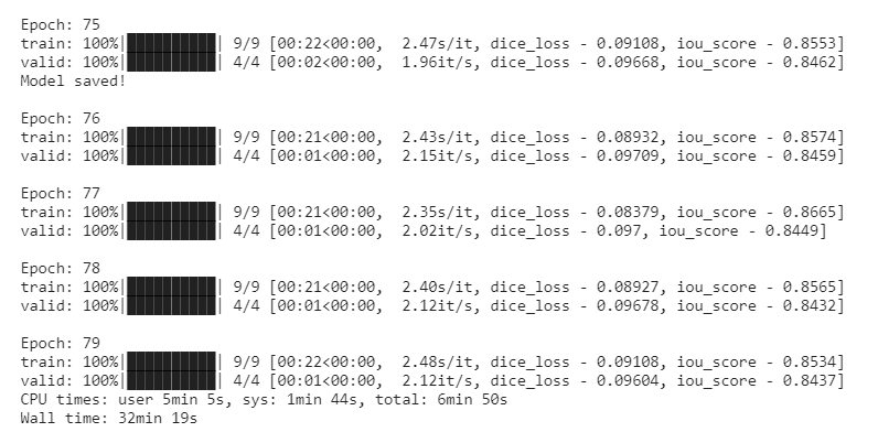
# Training DeepLabV3+
if TRAINING:
best_iou_score = 0.0
train_logs_list, valid_logs_list = [], []
for i in range(0, EPOCHS):
# Perform training & validation
print('\nEpoch: {}'.format(i))
train_logs = train_epoch.run(train_loader)
valid_logs = valid_epoch.run(valid_loader)
train_logs_list.append(train_logs)
valid_logs_list.append(valid_logs)
# Save model if a better val IoU score is obtained
if best_iou_score < valid_logs['iou_score']:
best_iou_score = valid_logs['iou_score']
torch.save(model, './best_model.pth')
print('Model saved!')
# Prediction on Test Data
# load best saved model checkpoint from the current run
if os.path.exists('./best_model.pth'):
best_model = torch.load('./best_model.pth', map_location=DEVICE)
print('Loaded DeepLabV3+ model from this run.')
# load best saved model checkpoint from previous commit (if present)
elif os.path.exists('../input//deeplabv3-efficientnetb4-frontend-using-pytorch/best_model.pth'):
best_model = torch.load('../input//deeplabv3-efficientnetb4-frontend-using-pytorch/best_model.pth', map_location=DEVICE)
print('Loaded DeepLabV3+ model from a previous commit.')
# create test dataloader (with preprocessing operation: to_tensor(...))
test_dataset = BuildingsDataset(
x_test_dir,
y_test_dir,
augmentation=get_validation_augmentation(),
preprocessing=get_preprocessing(preprocessing_fn),
class_rgb_values=select_class_rgb_values,
)
test_dataloader = DataLoader(test_dataset)
# test dataset for visualization (without preprocessing transformations)
test_dataset_vis = BuildingsDataset(
x_test_dir, y_test_dir,
augmentation=get_validation_augmentation(),
class_rgb_values=select_class_rgb_values,
)
# get a random test image/mask index
random_idx = random.randint(0, len(test_dataset_vis)-1)
image, mask = test_dataset_vis[random_idx]
visualize(
original_image = image,
ground_truth_mask = colour_code_segmentation(reverse_one_hot(mask), select_class_rgb_values),
one_hot_encoded_mask = reverse_one_hot(mask)
)
# Center crop padded image / mask to original image dims
def crop_image(image, target_image_dims=[1500,1500,3]):
target_size = target_image_dims[0]
image_size = len(image)
padding = (image_size - target_size) // 2
return image[
padding:image_size - padding,
padding:image_size - padding,
:,
]
sample_preds_folder = 'sample_predictions/'
if not os.path.exists(sample_preds_folder):
os.makedirs(sample_preds_folder)
for idx in range(len(test_dataset)):
image, gt_mask = test_dataset[idx]
image_vis = crop_image(test_dataset_vis[idx][0].astype('uint8'))
x_tensor = torch.from_numpy(image).to(DEVICE).unsqueeze(0)
# Predict test image
pred_mask = best_model(x_tensor)
pred_mask = pred_mask.detach().squeeze().cpu().numpy()
# Convert pred_mask from `CHW` format to `HWC` format
pred_mask = np.transpose(pred_mask,(1,2,0))
# Get prediction channel corresponding to building
pred_building_heatmap = pred_mask[:,:,select_classes.index('building')]
pred_mask = crop_image(colour_code_segmentation(reverse_one_hot(pred_mask), select_class_rgb_values))
# Convert gt_mask from `CHW` format to `HWC` format
gt_mask = np.transpose(gt_mask,(1,2,0))
gt_mask = crop_image(colour_code_segmentation(reverse_one_hot(gt_mask), select_class_rgb_values))
cv2.imwrite(os.path.join(sample_preds_folder, f"sample_pred_{idx}.png"), np.hstack([image_vis, gt_mask, pred_mask])[:,:,::-1])
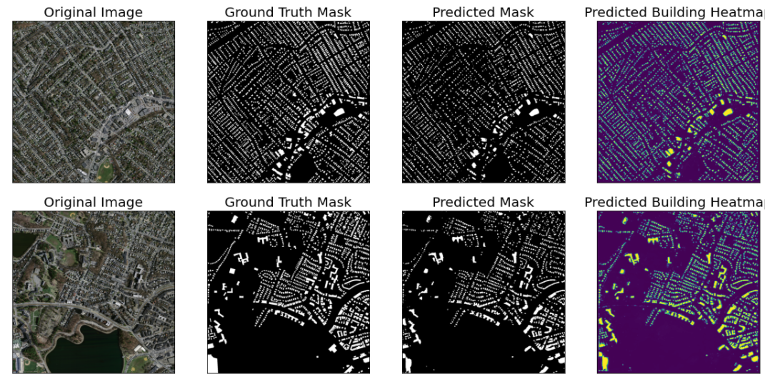
visualize(
original_image = image_vis,
ground_truth_mask = gt_mask,
predicted_mask = pred_mask,
predicted_building_heatmap = pred_building_heatmap
)
# Model Evaluation on Test Dataset
test_epoch = smp.utils.train.ValidEpoch(
model,
loss=loss,
metrics=metrics,
device=DEVICE,
verbose=True,
)
valid_logs = test_epoch.run(test_dataloader)
print("Evaluation on Test Data: ")
print(f"Mean IoU Score: {valid_logs['iou_score']:.4f}")
print(f"Mean Dice Loss: {valid_logs['dice_loss']:.4f}")
# Plot Dice Loss & IoU Metric for Train vs. Val
train_logs_df = pd.DataFrame(train_logs_list)
valid_logs_df = pd.DataFrame(valid_logs_list)
train_logs_df.T
plt.figure(figsize=(20,8))
plt.plot(train_logs_df.index.tolist(), train_logs_df.iou_score.tolist(), lw=3, label = 'Train')
plt.plot(valid_logs_df.index.tolist(), valid_logs_df.iou_score.tolist(), lw=3, label = 'Valid')
plt.xlabel('Epochs', fontsize=20)
plt.ylabel('IoU Score', fontsize=20)
plt.title('IoU Score Plot', fontsize=20)
plt.legend(loc='best', fontsize=16)
plt.grid()
plt.savefig('iou_score_plot.png')
plt.show()
plt.figure(figsize=(20,8))
plt.plot(train_logs_df.index.tolist(), train_logs_df.dice_loss.tolist(), lw=3, label = 'Train')
plt.plot(valid_logs_df.index.tolist(), valid_logs_df.dice_loss.tolist(), lw=3, label = 'Valid')
plt.xlabel('Epochs', fontsize=20)
plt.ylabel('Dice Loss', fontsize=20)
plt.title('Dice Loss Plot', fontsize=20)
plt.legend(loc='best', fontsize=16)
plt.grid()
plt.savefig('dice_loss_plot.png')
plt.show()
Visual presentation of raw data sets and labels
Training 80 epochs, model loss and segmentation score
Test and visualize results using test sets
Work summary of this week
1. The main idea of pseudolabel in the first paper is that entropy regularization has the same effect as pseudo label, and semi supervised learning can be carried out by using the information of the overlap degree of the distribution of unlabeled data.
2. The second paper, Mean Teacher, combines two other semi supervised learning models and methods( П- Model and Temporal ensembling) , the main idea is that there are two models: Student Model and teacher model. The teacher parameters are calculated by the student's exponential moving average value. The main purpose is to ensure that the prediction results of student model and teacher model are as similar as possible. Because the parameters of teacher model are obtained according to the moving average of student model, the prediction results are accurate for any new data There should not be too much jitter. If the model is correct, the prediction labels of the two models should be close, and the change is relatively small. Moving the model in the direction where the prediction results of the two models are close is moving in the direction of the growth truth model.
3. In the semantic segmentation task, the spatial pyramid pooling module (SPP) can capture more scale information, and the encoder decoder structure can better recover the edge information of the object. The DeepLabv3 + network uses both of the above points to build the network.