1. Picture loading, displaying and saving
cv2.imread(filename, flags): read and load images
cv2.imshow(winname, mat): displays a picture
cv2.waitKey(): wait for the picture to close
cv2.imwrite(filename, img): save the picture
2. Image display window creation and destruction
cv2.namedWindow(winname, attribute): create a window
cv2.destroyWindow(winname): destroy a window
cv2.destroyAllWindows(): destroy all windows
3. Acquisition of common attributes of pictures
img.shape: the height, width, and number of channels of the printed picture
img.size: number of pixels to print the picture
img.dtype: format for printing pictures
4. Select the rectangular region of interest (ROI)
A pixel of a picture can be represented by img[x, y, c] (x, y are coordinates and c is the number of channels)
A rectangular area of this picture can be represented as img[x1:x2, y1:y2, c] (the coordinates of the upper left corner of the rectangle are (x1, y1) and the coordinates of the lower right corner are (x2, y2))
Where the values of c are 0, 1 and 2 respectively for the corresponding B, G and R color channels, img[x, y] represents all channels by default
5. Separation and merging of picture color channels
cv2.split(img): separate the picture into three color channels
cv2.merge(img): merge three color channels into one picture
6. Picture two addition
cv2.add(src1, src2): normal addition
cv2.addWeighted(src1, alpha, src2, beta, gamma,dst): weighted addition
src1: first picture
alpha: weight of the first picture
src2: second picture
beta: weight of the second picture
gamma: the value added after the weighted addition of Figure 1 and Figure 2 (if the sum is greater than 255, it is pure white)
dst: output picture
7. Add & subtract & multiply & divide
def add_demo(m1, m2):
    dst = cv2.add(m1, m2) #plus
    cv2.imshow("add", dst)

def subtract_demo(m1, m2):
    dst = cv2.subtract(m1, m2) #reduce
    cv2.imshow("subtract", dst)

def multiply_demo(m1, m2):
    dst = cv2.multiply(m1, m2) #ride
    cv2.imshow("multiply", dst)

def divide_demo(m1, m2):
    dst = cv2.divide(m1, m2) #except
    cv2.imshow("divide", dst)
8. Mean & variance
def demo(img):
    M1 = cv2.mean(img)# mean value
    print(M1)
    M1, dev1 = cv2.meanStdDev(img) # Mean and variance
    print(M1)
    print(dev1)
9. And, or, not, XOR
def logic_demo(m1, m2):
    dst = cv2.bitwise_and(m1, m2) #And
    cv2.imshow("bitwise_and", dst)
    dst = cv2.bitwise_or(m1, m2) #or
    cv2.imshow("bitwise_or", dst)
    dst = cv2.bitwise_not(m1, m2) #Non (color flip)
    cv2.imshow("bitwise_not", dst)
    dst = cv2.bitwise_xor(m1, m2) #XOR
    cv2.imshow("bitwise_xor", dst)
10. Calculate execution time
cv2.getTickCount(): used to return the number of timing cycles that have elapsed since the operating system was started;
cv2.getTickFrequency(): used to return the CPU frequency, that is, the number of repetitions in one second.
time(s) = Total times / Number of repetitions in a second
 time(ms) = 1000 *Total times / Number of repetitions in a second
t1 = cv2.getTickCount()
function()   # Function to be tested
t2 = cv2.getTickCount()
time = (t2 - t1) / cv2.getTickFrequency()
print("time : %s ms" % (time * 1000))
11. Color space conversion
cv2.cvtColor(src,code,dst=None,dstCn=None)
Parameter: code, conversion type

# Color space conversion
def color_space_demo(img):
    gray = cv2.cvtColor(img, cv2.COLOR_BGR2GRAY)#BGR to GRAY
    cv2.imshow("gray", gray)
    hsv = cv2.cvtColor(img, cv2.COLOR_BGR2HSV)#BGR to HSV
    cv2.imshow("hsv", hsv)
    yuv = cv2.cvtColor(img, cv2.COLOR_BGR2YUV)#BGR to YUV
    cv2.imshow("yuv", yuv)
    ycrcb = cv2.cvtColor(img, cv2.COLOR_BGR2YCrCb)#BGR to CrCb
    cv2.imshow("ycrcb", ycrcb)
12. Mean fuzzy, median fuzzy, Gaussian fuzzy, bilateral fuzzy
cv2.blur()
Prototype: blur(src,ksize,dst=None,anchor=None,borderType=None)
Function: blur the arithmetic mean value of the image
Parameter: ksize, size of convolution kernel. dst. If dst is filled in, the image is written into the dst matrix
cv2.medianBlur()
Prototype: mediaBlur(src,ksize,dst=None)
Function: blur the median value of the image
cv2.GaussianBlur()
Prototype: Gaussian blur (SRC, ksize, sigma x, DST = none, sigma y = none, bordertype = none)
Function: Gaussian blur the image
Parameter: sigma x, variance in X direction, generally set to 0
cv2.bilateralFilter()
Prototype: bilaterfilter (SRC, D, sigma color, sigma space, DST = none, bordertype = none)
Function: blur the image bilaterally
Parameter: int d: indicates the diameter range of each pixel neighborhood in the filtering process. If the value is a non positive number, the function calculates the value from the fifth parameter sigmaSpace.
double sigmaColor: the sigma value of the color space filter. The larger the value of this parameter, the wider the colors in the pixel neighborhood will be mixed together to produce a larger semi equal color region.
Double sigma space: the Sigma value of the filter in the coordinate space. If the value is large, it means that the farther pixels will affect each other, so that enough similar colors in a larger area can obtain the same color. When d > 0, D specifies the neighborhood size and is independent of sigmaSpace, otherwise D is proportional to sigmaSpace
img = cv.imread('1.jpg',1)
blur = cv.blur(img,(5,5)) #Mean filtering
median = cv.medianBlur(img,5) #Median fuzzy
Gauss = cv.GaussianBlur(img,(5,5),0) #Gaussian blur
bilater = cv.bilateralFilter(img,9,75,75) #Bilateral ambiguity
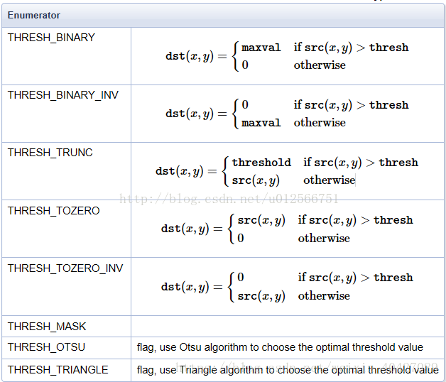
13. Binarization
Simple threshold operation
cv2.threshold()
Prototype: threshold (SRC, threshold, maxval, type, DST = none)
Function: binarize each pixel of the image
Parameter: thresh, threshold (minimum). maxval, the maximum value of binarization.
Type: binary type, which is generally set to 0, or the following values can be taken:

img = cv.imread('3.jpg',1)
gray = cv.cvtColor(img,cv2.COLOR_RGB2GRAY)
ret, thresh = cv.threshold(gray,127,255,cv.THRESH_BINARY)
Adaptive threshold operation
cv2.adaptiveThreshold(src, maxValue, adaptiveMethod, thresholdType, blockSize, C, dst=None)
Parameters:
maxValue: the maximum value of the threshold;
Adaptive method: Specifies the adaptive threshold algorithm; Specific parameters can be selected as follows:
     ADAPTIVE_THRESH_MEAN_C: Is the average of local neighborhood blocks. The algorithm first obtains the mean value in the block, and then subtracts the constant C.
     ADAPTIVE_THRESH_GAUSSIAN_C: Is the Gaussian weighted sum of local neighborhood blocks. The algorithm is in the region( x,y)The surrounding pixels are weighted according to their distance from the center according to the Gaussian function, and then the constant is subtracted C.
thresholdType: Specifies the threshold type. You can select either THRESH_BINARY or THRESH_BINARY_INV. (i.e. binary threshold or anti binary threshold).
blockSize: indicates the size of the neighborhood block. It is used to calculate the region threshold. It is an odd number. Generally, it is 3, 5, 7, etc.
C: Represents the parameter related to the algorithm. It is a constant extracted from the mean or weighted mean, which can be negative.
# Local binarization
def local_threshold_demo():
    gray = cv2.cvtColor(img, cv2.COLOR_BGR2GRAY)
    binary = cv2.adaptiveThreshold(gray, 255, cv2.ADAPTIVE_THRESH_MEAN_C, cv2.THRESH_BINARY, 25, 10)
    #print("threshold value : %s\n" % ret)
    cv2.imshow("binary_local", binary)
14. Image histogram
CV2. Calchist (images, channels, mask, histsize, ranges [, hist [, aggregate]]) draws histograms
cv2.equalizeHist(img) histogram equalization
Parameters:
images: (input image) parameters must be enclosed in square brackets.
channels: calculate the channel of the histogram.
Mask: (mask), generally used as None, indicates processing the whole image.
histSize: indicates how many parts the histogram is divided into (i.e. how many square columns).
range: the value of each pixel in the histogram, [0.0, 256.0] indicates that the histogram can represent pixels with pixel values from 0.0 to 256.
Finally, there are two optional parameters. Since the histogram is returned as a function result, the sixth hist is meaningless (to be determined). The last accumulate is a Boolean value to indicate whether the histogram is superimposed.
img = cv.imread('3.jpg', 0)
hist = cv.calcHist([img], [0], None, [256], [0, 256])  # Draw histogram
equ = cv.equalizeHist(img) #Histogram equalization
15. Template matching
matchTemplate(image, templ, method, result=None, mask=None)
Parameters:
Image: source image S;
templ: template image T, generally a small piece of source image S;
method: template matching algorithm (cv.tm_sqdiff_normalized is the most similar when it is the smallest, and the most similar when it is the largest)
# 1 image and template reading
img = cv.imread('1.jpg')
template = cv.imread('1_1.jpg')
h,w,l = template.shape
# 2 template matching
# 2.1 template matching
res = cv.matchTemplate(img, template, cv.TM_CCOEFF)
# 2.2 return the most matched position in the image, determine the coordinates of the upper left corner, and draw the matching position on the image
min_val, max_val, min_loc, max_loc = cv.minMaxLoc(res)
top_left = max_loc
bottom_right = (top_left[0] + w, top_left[1] + h)
cv.rectangle(img, top_left, bottom_right, (0,255,0), 2)
# 3 image display
plt.ims
how(img[:,:,::-1])
plt.title('Matching results'), plt.xticks([]), plt.yticks([])
plt.show()


16. Image pyramid (upsampling and downsampling)
Downsampling image reduction (Gaussian blur first, and then downsampling, which needs to be repeated again and again, not to the end at one time)
Upsampling image expansion (first expansion, then convolution, or use Laplacian pyramid)
17,Soble&scharr&Laplacian
cv2.Sobel()
Prototype: Sobel(src,ddepth,dx,dy,dst=None,ksize=None,scale=None,delta=None,borderType=None)
Function: calculate the Sobel operator of the image and detect its edge.
Parameters:
dx: derivative order in x direction;
dy: derivative order in the y direction.
#-------------------------Soble operator--------------------------
# 1 read image
img = cv.imread('2.jpg',0)
# 2 calculate Sobel convolution results
x = cv.Sobel(img, cv.CV_16S, 1, 0)
y = cv.Sobel(img, cv.CV_16S, 0, 1)
# 3 convert data
Scale_absX = cv.convertScaleAbs(x)  # convert scale
Scale_absY = cv.convertScaleAbs(y)
# 4 Result synthesis
result = cv.addWeighted(Scale_absX, 0.5, Scale_absY, 0.5, 0)
cv2.scharr()
Prototype: Scharr(src, ddepth, dx, dy, dst=None, scale=None, delta=None, borderType=None, /)
Parameters:
src: original image
ddepth: processing result image depth
dx: x-axis direction
dy: y-axis direction
cv2.Laplacian()
Prototype: Laplacian(src,ddepth,dst=None,ksize=None,scale=None,delta=None,borderType=None)
Function: detect image edges.
Parameters:
ddepth: image bit depth. For grayscale images, its value is cv2.CV_8U. ksize, the size of the convolution kernel you want to use. scale: is the scaling constant of the scaling derivative.
#-------------------------Laplacian operator--------------------------
# 1 read image
img2 = cv.imread('2.jpg',0)
# 2 laplacian conversion
result = cv.Laplacian(img2,cv.CV_16S)
Scale_abs = cv.convertScaleAbs(result)
# 3 image display