Computer vision is one of the most popular fields in the current industry. With the rapid development of technology and research, it is booming. But it's still a tough task for newcomers. There are some common challenges for the developers or data scientists of XR R in their transition to computer vision, including:
1. How do we clean up image data sets? Images have different shapes and sizes
2. Problems in data acquisition. Should we collect more images before building a computer vision model?
3. Is deep learning essential for building computer vision model? Can we not use machine learning technology?
4. Can we build computer vsiion model on our own machine? Not everyone can use GPU and TPU!
The following is the official account: AIRX community (domestic leading AI, AR, VR technology learning and communication platform).
Catalog
-
What is computer vision?
-
Why use OpenCV for computer vision tasks?
-
Read, write and display images
-
Change color space
-
Resize image
-
Image rotation
-
Picture translation
-
Simple image threshold
-
Adaptive threshold
-
Image segmentation (watershed algorithm)
-
Bitwise operation
-
edge detection
-
Image filtering
-
Image outline
-
Scale invariant feature transformation (SIFT)
-
Power of acceleration (SURF)
-
Feature matching
-
Face detection
What is CV
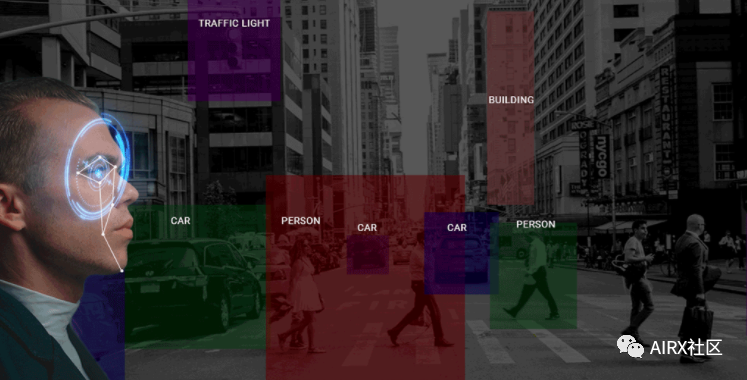
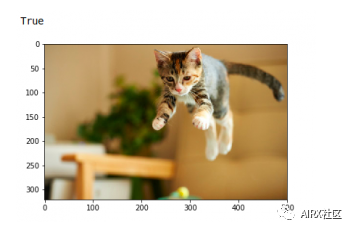
Before entering OpenCV, let me quickly explain what computer vision is. Have an intuitive understanding of what will be discussed in the rest of this article. Human beings can see and perceive the world naturally. It's our second nature to gather information from our surroundings through the gift of vision and perception.
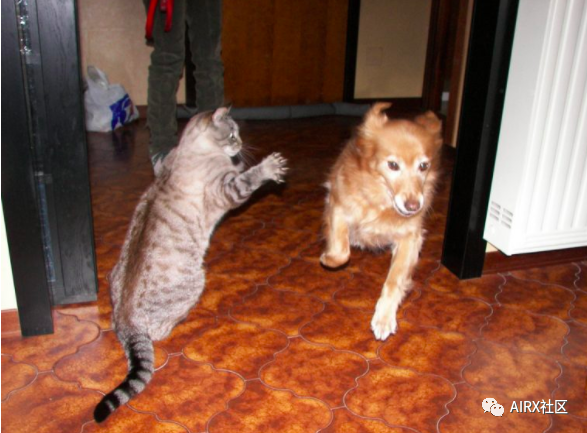
Take a quick look at the image above. It took us less than a second to find out that there was a cat, a dog and a human leg. For machines, this learning process becomes very complicated. The process of image analysis and object detection involves many complex steps, including feature extraction (edge detection, shape, etc.), feature classification, etc.
Computer vision is one of the most popular fields in the current industry. It can be predicted that there will be a large number of vacancies in the next two to four years. So the question is are you ready to take advantage of these opportunities? Take a moment to think about it - what applications or products do you think about when you think about computer vision? We use some of them every day, using facial recognition to unlock mobile phone, mobile phone camera, self driving car and so on.
About OpenCV
OpenCV library was originally a research project of Intel. As far as its functions are concerned, it is the largest computer vision library at present. OpenCV contains more than 2500 algorithms! It can be used for free for commercial and academic purposes. The library has interfaces for multiple languages, including Python, Java, and C + +.
The first version of OpenCV, 1.0, was released in 2006, and the opencv community has grown rapidly since then.
Now, let's turn our attention to the idea behind this article - the many features OpenCV offers! We'll look at OpenCV from a data scientist's point of view and learn about features that make it easier to develop and understand computer vision models.
Read, write and display images
The machine uses numbers to view and process everything, including images and text. How do you convert images into numbers? Yes, pixels!
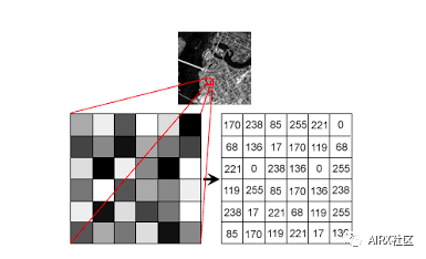
Each number represents the pixel strength for that particular location. In the image above, I show the pixel values of a grayscale image, where each pixel contains only one value, the black intensity of the location.
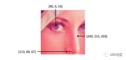
Note that color images have multiple values for a single pixel. These values represent the intensity of each channel - for example, the red, green, and blue channels of an RGB image.
Reading and writing images is an essential part of any computer vision project. The OpenCV library makes this function very simple.
#import the librariesimport numpy as npimport matplotlib.pyplot as pltimport cv2%matplotlib inline#reading the imageimage = cv2.imread('index.png')image = cv2.cvtColor(image,cv2.COLOR_BGR2RGB)#plotting the imageplt.imshow(image)#saving imagecv2.imwrite('test_write.jpg',image)
By default, the imread function reads the image in BGR (cyan red) format. We can use the extra flags in the imread function to read images in different formats:
-
Cv2.imread'color: default flag for loading color images
-
Cv2.imread'grayscale: load image in grayscale format
-
Cv2.imread_unhanged: loads an image in the given format, including the alpha channel. Alpha channel stores transparency information. The higher the value of alpha channel, the more opaque the pixel.
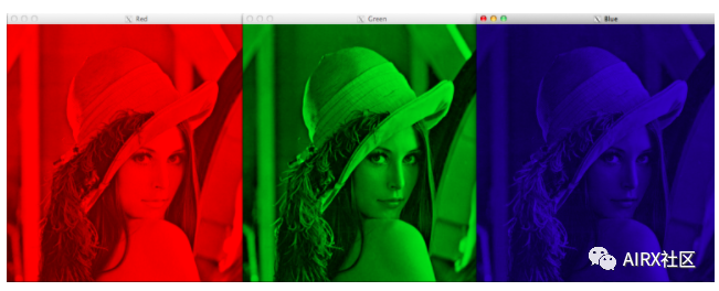
Change color space
Color space is a protocol for representing colors in a way that makes them easy to copy. We know that gray-scale image has a single pixel value, while color image contains three values for each pixel - the intensity of red, green and blue channels.
Most computer vision use cases process RGB images. However, applications such as video compression and device independent storage rely heavily on other color spaces, such as color saturation values or HSV color spaces.
As you understand, RGB image is composed of color intensity of different color channels, that is, intensity and color information are mixed in RGB color space, while in HSV color space, color and intensity information are separated from each other. This makes the HSV color space more robust to light changes. Opencv reads the given image in BGR format by default. Therefore, when using OpenCV to read an image, you need to change the color space of the image from BGR to RGB. Let's see how:
#import the required librariesimport numpy as npimport matplotlib.pyplot as pltimport cv2%matplotlib inlineimage = cv2.imread('index.jpg')#converting image to Gray scalegray_image = cv2.cvtColor(image,cv2.COLOR_BGR2GRAY)#plotting the grayscale imageplt.imshow(gray_image)#converting image to HSV formathsv_image = cv2.cvtColor(image,cv2.COLOR_BGR2HSV)#plotting the HSV imageplt.imshow(hsv_image)
Resize image
The machine learning model works with fixed size input. The same idea applies to computer vision models. The image we use to train the model must be the same size.
Now, if we create our own datasets by grabbing images from various sources, this can be a problem. This is the ability to resize the image.
Opencv makes it easy to zoom in and out of images. When we need to transform the image into the input shape of the model, this operation is very useful for training the deep learning model. OpenCV supports different interpolation and down sampling methods, and these parameters can be used by the following parameters:
1. Inter ﹣ nearest neighbor interpolation
2. Inter? Linear: bilinear interpolation
3. Inter? Area: resampling using pixel area relationship
4. Intercubic: bicubic interpolation on 4 × 4 pixel neighborhood
5. Interczos interpolation in 8 × 8 neighborhood
OpenCV's resize feature uses bilinear interpolation by default.
import cv2import numpy as npimport matplotlib.pyplot as plt%matplotlib inline#reading the imageimage = cv2.imread('index.jpg')#converting image to size (100,100,3)smaller_image = cv2.resize(image,(100,100),inerpolation='linear')#plot the resized imageplt.imshow(smaller_image)
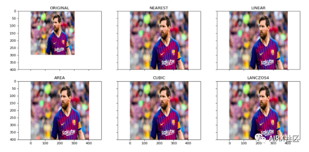
Image rotation
"You need a lot of data to train deep learning models.". Most deep learning algorithms depend on the quality and quantity of data to a great extent. But what if you don't have a large enough dataset? Not everyone can afford to manually collect and tag images.
Suppose we are building an image classification model to identify the animals in the image. Therefore, both images shown below should be classified as "dogs":
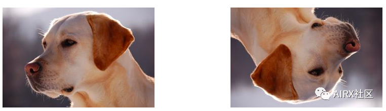
However, if the second image is not trained, the model may find it difficult to classify it as a dog. So what should we do?
Let me introduce data expansion technology. This method allows us to generate more samples to train our deep learning model. Data expansion uses existing data samples to generate new data samples by applying image operations such as rotation, zoom, translation, etc. This makes our model robust to input changes and leads to better generalization.
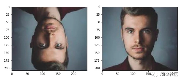
Rotation is one of the most commonly used and easily implemented data expansion technologies. As the name implies, it includes rotating the image at any angle and providing it with the same label as the original image. Think about how many times you rotate an image in your phone to achieve an angle - that's basically what this function does.
#importing the required librariesimport numpy as npimport cv2import matplotlib.pyplot as plt%matplotlib inlineimage = cv2.imread('index.png')rows,cols = image.shape[:2]#(col/2,rows/2) is the center of rotation for the image# M is the cordinates of the centerM = cv2.getRotationMatrix2D((cols/2,rows/2),90,1)dst = cv2.warpAffine(image,M,(cols,rows))plt.imshow(dst)
Picture translation
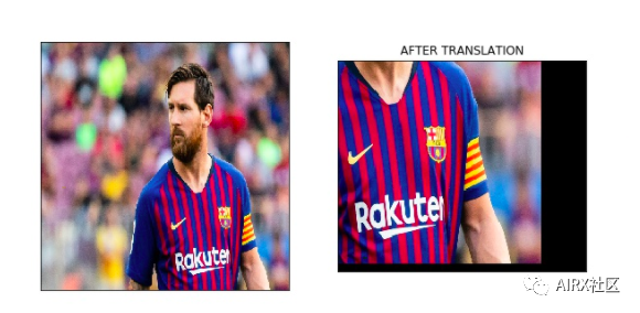
Image translation is a geometric transformation that maps the position of each object in the image to a new position in the final output image. After the pan operation, the object at the position (x, y) in the input image moves to the new position (x, y):
X = x + dx
Y = y + dy
Here, dx and dy are the respective translations along different dimensions. Image translation can be used to add translation invariance to the model, because through translation, we can change the position of the object in the image, so that the model has more diversity, which leads to better generalization.
Take the picture below as an example. Even if there is no complete shoe in the image, the model should be able to classify it as a shoe.
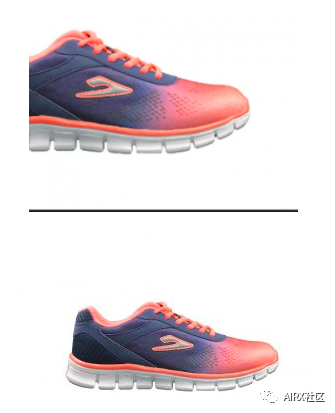
This conversion function is usually used in the image preprocessing stage. Look at the following code to see how it works in practice:
#importing the required librariesimport numpy as npimport cv2import matplotlib.pyplot as plt%matplotlib inline#reading the imageimage = cv2.imread('index.png')#shifting the image 100 pixels in both dimensionsM = np.float32([[1,0,-100],[0,1,-100]])dst = cv2.warpAffine(image,M,(cols,rows))plt.imshow(dst)
Simple image threshold
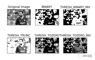
Thresholding is an image segmentation method. It compares pixel values with thresholds and updates them accordingly. OpenCV supports a variety of threshold changes. A simple threshold function can be defined as follows:
If Image (x, y) > threshold, Image (x, y) = 1
Otherwise, Image (x, y) = 0
Thresholds can only be applied to grayscale images. A simple application of image thresholding is to divide image into foreground and background.
#importing the required librariesimport numpy as npimport cv2import matplotlib.pyplot as plt%matplotlib inline#here 0 means that the image is loaded in gray scale formatgray_image = cv2.imread('index.png',0)ret,thresh_binary = cv2.threshold(gray_image,127,255,cv2.THRESH_BINARY)ret,thresh_binary_inv = cv2.threshold(gray_image,127,255,cv2.THRESH_BINARY_INV)ret,thresh_trunc = cv2.threshold(gray_image,127,255,cv2.THRESH_TRUNC)ret,thresh_tozero = cv2.threshold(gray_image,127,255,cv2.THRESH_TOZERO)ret,thresh_tozero_inv = cv2.threshold(gray_image,127,255,cv2.THRESH_TOZERO_INV)#DISPLAYING THE DIFFERENT THRESHOLDING STYLESnames = ['Oiriginal Image','BINARY','THRESH_BINARY_INV','THRESH_TRUNC','THRESH_TOZERO','THRESH_TOZERO_INV']images = gray_image,thresh_binary,thresh_binary_inv,thresh_trunc,thresh_tozero,thresh_tozero_invfor i in range(6):plt.subplot(2,3,i+1),plt.imshow(images[i],'gray')plt.title(names[i])plt.xticks([]),plt.yticks([])plt.show()
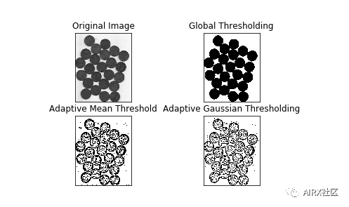
Adaptive threshold
In the case of adaptive thresholds, different thresholds are used for different parts of the image. This function can provide better results for images with varying lighting conditions, so it is called "adaptive". Otsu's binary method finds the best threshold for the whole image. It is suitable for bimodal image (image with 2 peaks in histogram).
#import the librariesimport numpy as npimport matplotlib.pyplot as pltimport cv2%matplotlib inline#ADAPTIVE THRESHOLDINGgray_image = cv2.imread('index.png',0)ret,thresh_global = cv2.threshold(gray_image,127,255,cv2.THRESH_BINARY)#here 11 is the pixel neighbourhood that is used to calculate the threshold valuethresh_mean = cv2.adaptiveThreshold(gray_image,255,cv2.ADAPTIVE_THRESH_MEAN_C,cv2.THRESH_BINARY,11,2)thresh_gaussian = cv2.adaptiveThreshold(gray_image,255,cv2.ADAPTIVE_THRESH_GAUSSIAN_C,cv2.THRESH_BINARY,11,2)names = ['Original Image','Global Thresholding','Adaptive Mean Threshold','Adaptive Gaussian Thresholding']images = [gray_image,thresh_global,thresh_mean,thresh_gaussian]for i in range(4):plt.subplot(2,2,i+1),plt.imshow(images[i],'gray')plt.title(names[i])plt.xticks([]),plt.yticks([])plt.show()
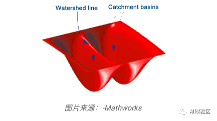
Image segmentation (watershed algorithm)
Image segmentation is the task of classifying every pixel in an image into a certain class. For example, classify each pixel as a foreground or background. Image segmentation is very important to extract relevant parts from image.
Watershed algorithm is a classical image segmentation algorithm. It treats pixel values in the image as terrain. To find the object boundary, it takes the initial tag as input. Then, the algorithm starts from the flood basin in the marker until the marker meets at the object boundary.
Suppose we have multiple basins. Now, if we fill different basins with different colors of water, the intersection of different colors will provide us with object boundaries.
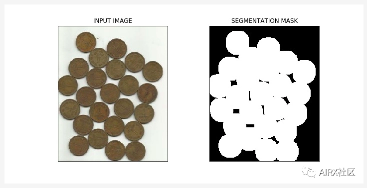
#importing required librariesimport numpy as npimport cv2import matplotlib.pyplot as plt#reading the imageimage = cv2.imread('coins.jpg')#converting image to grayscale formatgray = cv2.cvtColor(image,cv2.COLOR_BGR2GRAY)#apply thresholdingret,thresh = cv2.threshold(gray,0,255,cv2.THRESH_BINARY_INV+cv2.THRESH_OTSU)#get a kernelkernel = np.ones((3,3),np.uint8)opening = cv2.morphologyEx(thresh,cv2.MORPH_OPEN,kernel,iterations = 2)#extract the background from imagesure_bg = cv2.dilate(opening,kernel,iterations = 3)dist_transform = cv2.distanceTransform(opening,cv2.DIST_L2,5)ret,sure_fg = cv2.threshold(dist_transform,0.7*dist_transform.max(),255,0)sure_fg = np.uint8(sure_fg)unknown = cv2.subtract(sure_bg,sure_bg)ret,markers = cv2.connectedComponents(sure_fg)markers = markers+1markers[unknown==255] = 0markers = cv2.watershed(image,markers)image[markers==-1] = [255,0,0]plt.imshow(sure_fg)
Transposition operation
Bitwise operations include AND, OR, NOT, AND XOR. You may remember them in programming class! In computer vision, these operations are very useful when we have a mask image AND want to apply the mask to another image to extract the region of interest.
#import required librariesimport numpy as npimport matplotlib.pyplot as pltimport cv2%matplotlib inline#read the imageimage = cv2.imread('coins.jpg')#apply thresholdinret,mask = cv2.threshold(sure_fg,0,255,cv2.THRESH_BINARY_INV+cv2.THRESH_OTSU)#apply AND operation on image and mask generated by thrresholdingfinal = cv2.bitwise_and(image,image,mask = mask)#plot the resultplt.imshow(final)
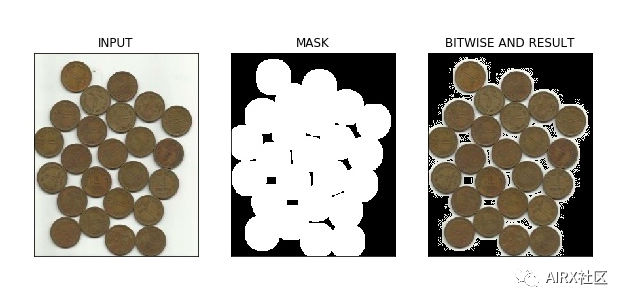
In the figure above, we can see the input image calculated by watershed algorithm and its segmentation mask. In addition, we apply the bitwise and operation to remove the background from the image and extract relevant parts from the image.
edge detection
An edge is a point in an image where the brightness of the image changes rapidly or is not continuous. This discontinuity usually corresponds to:
-
Depth discontinuity
-
Discontinuity of surface orientation
-
Changes in material properties
-
Changes in scene lighting
Edge is a very useful function of image, which can be used in different applications, such as object classification and positioning in image. Even the deep learning model computes edge features to extract information about the objects in the image.
Edges and contours are different because they are not related to objects, but represent changes in the pixel values of the image. Edge detection can be used for image segmentation or even image sharpening.
#import the required librariesimport numpy as np import cv2 import matplotlib.pyplot as plt %matplotlib inline#read the imageimage = cv2.imread('coins.jpg') #calculate the edges using Canny edge algorithmedges = cv2.Canny(image,100,200) #plot the edgesplt.imshow(edges)
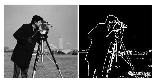
Image filtering
In image filtering, the pixel value is updated with the neighboring value of the pixel. But how do these values update first?
Well, there are many ways to update the pixel value, such as selecting the maximum value from the neighbors, using the average value of the neighbors, and so on. Each method has its own purpose. For example, pixel values in the neighborhood are averaged for image blur.
Gaussian filtering is also used for image blur, which gives different weights to neighboring pixels based on their distance from the considered pixels.
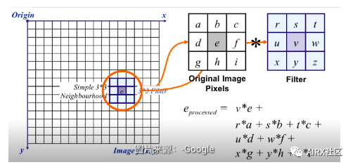
For image filtering, we use the kernel. The kernel is a digital matrix with different shapes, such as 3 x 3, 5 x 5, etc. The kernel is used to calculate the dot product with a part of the image. When calculating a new value for a pixel, the center of the kernel overlaps the pixel. The adjacent pixel values are multiplied by the corresponding values in the kernel. Assign the calculated value to the pixels consistent with the kernel center.
#importing the required libraries import numpy as np import cv2 import matplotlib.pyplot as plt %matplotlib inline image = cv2.imread('index.png') #using the averaging kernel for image smoothening averaging_kernel = np.ones((3,3),np.float32)/9 filtered_image = cv2.filter2D(image,-1,kernel) plt.imshow(dst) #get a one dimensional Gaussian Kernel gaussian_kernel_x = cv2.getGaussianKernel(5,1) gaussian_kernel_y = cv2.getGaussianKernel(5,1) #converting to two dimensional kernel using matrix multiplication gaussian_kernel = gaussian_kernel_x * gaussian_kernel_y.T #you can also use cv2.GaussianBLurring(image,(shape of kernel),standard deviation) instead of cv2.filter2D filtered_image = cv2.filter2D(image,-1,gaussian_kernel) plt.imshow()
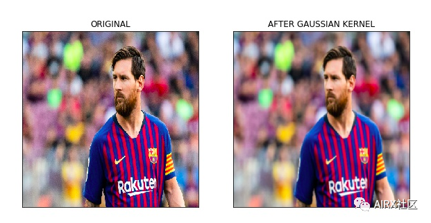
In the above output, the image on the right shows the result of applying Gaussian kernel on the input image. We can see that the edges of the original image are suppressed. Gaussian kernels with different sigma values are widely used to calculate the Gaussian difference of our images. This is an important step in the process of feature extraction, because it can reduce the noise in the image.
Image outline
A profile is a closed curve of a point or segment that represents the boundary of an object in an image. The outline is essentially the shape of the object in the image.
Unlike the edge, the outline is not part of the image. Instead, they are abstract collections of points and line segments corresponding to the shape of the object in the image.
We can use contour to calculate the number of objects in the image, classify objects according to their shapes, or select objects with specific shapes from the image.
#importing the required libraries import numpy as np import cv2 import matplotlib.pyplot as plt %matplotlib inline image = cv2.imread('shapes.png') #converting RGB image to Binary gray_image = cv2.cvtColor(image,cv2.COLOR_BGR2GRAY) ret,thresh = cv2.threshold(gray_image,127,255,0) #calculate the contours from binary imageim,contours,hierarchy = cv2.findContours(thresh,cv2.RETR_TREE,cv2.CHAIN_APPROX_SIMPLE) with_contours = cv2.drawContours(image,contours,-1,(0,255,0),3) plt.imshow(with_contours)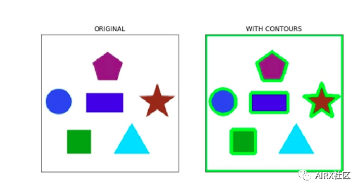
Scale invariant feature transformation (SIFT)
The key point is the concept that should be paid attention to when processing the image. These are basically the concerns in the image. The key points are similar to the features of a given image.
They are the places where interesting content in an image is defined. Key points are important because we always find the same key points for the image regardless of how we modify the image (rotate, shrink, expand, deform).
Scale invariant feature transform (SIFT) is a very popular key point detection algorithm. It includes the following steps:
-
Extremum detection in scale space
-
Key localization
-
Direction assignment
-
Key descriptor
-
Key matching
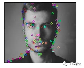
The features extracted from SIFT can be used in image mosaic, object detection and other applications. The following code and output show the key and its direction calculated using sift.
#import required librariesimport cv2import numpy as npimport matplotlib.pyplot as plt%matplotlib inline#show OpenCV versionprint(cv2.__version__)#read the iamge and convert to grayscaleimage = cv2.imread('index.png')gray = cv2.cvtColor(image,cv2.COLOR_BGR2GRAY)#create sift objectsift = cv2.xfeatures2d.SIFT_create()#calculate keypoints and their orientationkeypoints,descriptors = sift.detectAndCompute(gray,None)#plot keypoints on the imagewith_keypoints = cv2.drawKeypoints(gray,keypoints)#plot the imageplt.imshow(with_keypoints)
SURF
SURF is an enhanced version of SIFT. It works faster and is more robust for image conversion. In SIFT, the scale space is approximated by the Laplace operator of Gauss. What is the Laplace operator of Gauss?
Laplace operator is the kernel used to calculate image edge. The Laplace kernel works by approximating the second derivative of the image. Therefore, it is very sensitive to noise. We usually apply Gauss kernel to the image before Laplace kernel, so we call it Gauss Laplace.
In SURF, the Laplacian operator of Gauss is calculated by using a box filter (kernel). The convolution of the box filter can be carried out in parallel for different proportions, which is the root cause of the increase of SURF speed (compared with SIFT).
#import required librariesimport cv2import numpy as npimport matplotlib.pyplot as plt%matplotlib inline#show OpenCV versionprint(cv2.__version__)#read image and convert to grayscaleimage = cv2.imread('index.png')gray = cv2.cvtColor(image,cv2.COLOR_BGR2GRAY)#instantiate surf objectsurf  = cv2.xfeatures2d.SURF_create(400)#calculate keypoints and their orientationkeypoints,descriptors = surf.detectAndCompute(gray,None)
with_keypoints = cv2.drawKeypoints(gray,keypoints)
plt.imshow(with_keypoints)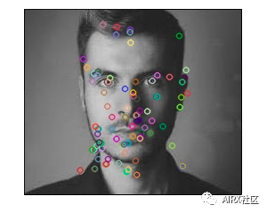
Feature matching
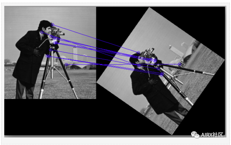
Features extracted from different images using SIFT or SURF can be matched to find similar objects / patterns in different images. OpenCV library supports a variety of functional matching algorithms, such as brute force matching, knn feature matching and so on.
import numpy as npimport cv2import matplotlib.pyplot as plt%matplotlib inline#reading images in grayscale formatimage1 = cv2.imread('messi.jpg',0)image2 = cv2.imread('team.jpg',0)#finding out the keypoints and their descriptorskeypoints1,descriptors1 = cv2.detectAndCompute(image1,None)keypoints2,descriptors2 = cv2.detectAndCompute(image2,None)#matching the descriptors from both the imagesbf = cv2.BFMatcher()matches = bf.knnMatch(ds1,ds2,k = 2)#selecting only the good featuresgood_matches = []for m,n in matches:if m.distance < 0.75*n.distance:good.append([m])image3 = cv2.drawMatchesKnn(image1,kp1,image2,kp2,good,flags = 2)
In the above image, we can see that the key extracted from the original image (on the left) matches the key of its rotation version. This is because the feature is used SIFT Extracted, and SIFT It is invariant for such transformations.
Face detection
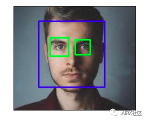
OpenCV Support based on haar Cascaded object detection. Haar Cascading is a classifier based on machine learning, which can calculate different features (such as edges, lines, etc.) in images. Then, these classifiers are trained with multiple positive and negative samples.
OpenCV Github The repository provides training classifiers for different objects (such as face, eyes, etc.), and you can also train your own for any object haar Cascade.
#import required librariesimport numpy as npimport cv2 as cvimport matplotlib.pyplot as plt%matplotlib inline#load the classifiers downloadedface_cascade = cv.CascadeClassifier('haarcascade_frontalface_default.xml')eye_cascade = cv.CascadeClassifier('haarcascade_eye.xml')#read the image and convert to grayscale formatimg = cv.imread('rotated_face.jpg')gray = cv.cvtColor(img, cv.COLOR_BGR2GRAY)#calculate coordinatesfaces = face_cascade.detectMultiScale(gray, 1.1, 4)for (x,y,w,h) in faces:cv.rectangle(img,(x,y),(x+w,y+h),(255,0,0),2)roi_gray = gray[y:y+h, x:x+w]roi_color = img[y:y+h, x:x+w]eyes = eye_cascade.detectMultiScale(roi_gray)#draw bounding boxes around detected featuresfor (ex,ey,ew,eh) in eyes:cv.rectangle(roi_color,(ex,ey),(ex+ew,ey+eh),(0,255,0),2)#plot the imageplt.imshow(img)#write imagecv2.imwrite('face_detection.jpg',img)
As for more machine learning, AI, augmented reality resources and technology dry cargo, we can pay attention to the official account: AIRX community, learn together and make progress together!