In recent years, with the rapid development of information technology, intelligent devices are gradually integrated into people's daily life. As one of the most convenient ways of human-computer interaction, voice has been widely used. It is the goal of countless researchers to make machines understand human language and realize the natural communication with human beings. The main content of speech emotion recognition is to establish a computing system that can analyze and recognize human emotion from speech, and realize the human communication between human and machine.
The main task of speech emotion recognition is to extract the emotion information contained in speech and recognize its category. At present, there are two ways to describe emotion. The first is based on the discrete emotion division, which divides the basic emotions widely used in human daily life into anger, happiness, excitement, sadness, disgust, etc.; the other is based on the continuous dimension emotion division, mainly through different potency and activation degree to distinguish different emotions.
As a classification task, feature selection is the most critical step. The speech feature used in this paper is Mel cepstrum coefficient. For the knowledge of what Mel cepstrum coefficient is and how to extract it, please refer to the article Python voice signal processing.
This paper refers to MITESHPUTHRANNEU/Speech-Emotion-Analyzer In this project, we will start to introduce how to analyze voice emotion through convolutional neural network
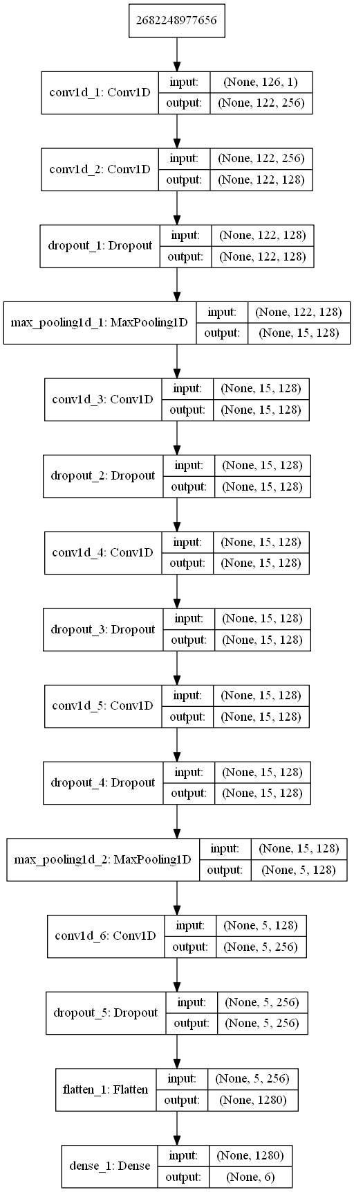
Neural network structure
The architecture used is very simple, as follows
data set
I used CASIA's voice emotion database. CASIA Chinese emotional corpus was recorded by the Institute of Automation, Chinese Academy of Sciences. It consists of four professional speakers, six kinds of emotional angry, happy, fear, sad, surprise and neutral, with 9600 different pronunciations. Among them, 300 sentences are of the same text, that is to say, the same text is read with different emotions. These corpora can be used to compare and analyze the acoustic and rhythmic performance under different emotional states; the other 100 sentences are of different texts, and their emotional attribution can be seen from the literal meaning of these texts, so that the recorder can more accurately express his emotions.
But the complete CASIA dataset is charged, so I only found 1200 incomplete datasets. I put the dataset I found on my network disk: https://pan.baidu.com/s/1EsRoKaF17Q_3s2t7OMNibQ.
feature extraction
I use librosa module to extract MFCC. The extraction code is as follows.
%matplotlib inline
import librosa
import matplotlib.pyplot as plt
import numpy as np

path=r'D:\NLP\dataset\Voice emotion\test.wav'

y,sr = librosa.load(path,sr=None)

def normalizeVoiceLen(y,normalizedLen):
    nframes=len(y)
    y = np.reshape(y,[nframes,1]).T
    #Normalized audio length is 2s,32000 data points
    if(nframes<normalizedLen):
        res=normalizedLen-nframes
        res_data=np.zeros([1,res],dtype=np.float32)
        y = np.reshape(y,[nframes,1]).T
        y=np.c_[y,res_data]
    else:
        y=y[:,0:normalizedLen]
    return y[0]

def getNearestLen(framelength,sr):
    framesize = framelength*sr
    #Find the positive integer power of 2 closest to the current framesize
    nfftdict = {}
    lists = [32,64,128,256,512,1024]
    for i in lists:
        nfftdict[i] = abs(framesize - i)
    sortlist = sorted(nfftdict.items(), key=lambda x: x[1])#In ascending order of difference from current framesize
    framesize = int(sortlist[0][0])#Take the positive integer power of the 2 closest to the current framesize as the new framesize
    return framesize

VOICE_LEN=32000
#Get n_ Length of FFT
N_FFT=getNearestLen(0.25,sr)
#Unified sound range is the first two seconds
y=normalizeVoiceLen(y,VOICE_LEN)
print(y.shape)
#Extract mfcc features
mfcc_data=librosa.feature.mfcc(y=y, sr=sr,n_mfcc=13,n_fft=N_FFT,hop_length=int(N_FFT/4))

# Draw a feature map to visualize MFCC. Transpose the matrix so that the time domain is horizontal
plt.matshow(mfcc_data)
plt.title('MFCC')
The function of the above code is to load the sound and take the first two seconds of the sound for emotional analysis. The getNearestLen() function determines an appropriate speech frame length for Fourier transform based on the sampling rate of the voice. And then through librosa.feature.mfcc The () function extracts MFCC features and visualizes them.
The following code extracts the mfcc features from the dataset, averages the mfcc of each frame, and saves the result as a file.
#Extract features
import os
import pickle

counter=0
fileDirCASIA = r'./Voice emotion/CASIA database'

mfccs={}
mfccs['angry']=[]
mfccs['fear']=[]
mfccs['happy']=[]
mfccs['neutral']=[]
mfccs['sad']=[]
mfccs['surprise']=[]
mfccs['disgust']=[]

listdir=os.listdir(fileDirCASIA)
for persondir in listdir:
    if(not r'.' in persondir):
        emotionDirName=os.path.join(fileDirCASIA,persondir)
        emotiondir=os.listdir(emotionDirName)
        for ed in emotiondir:
            if(not r'.' in ed):
                filesDirName=os.path.join(emotionDirName,ed)
                files=os.listdir(filesDirName)
                for fileName in files:
                    if(fileName[-3:]=='wav'):
                        counter+=1
                        fn=os.path.join(filesDirName,fileName)
                        print(str(counter)+fn)
                        y,sr = librosa.load(fn,sr=None)
                        y=normalizeVoiceLen(y,VOICE_LEN)#Normalized length
                        mfcc_data=librosa.feature.mfcc(y=y, sr=sr,n_mfcc=13,n_fft=N_FFT,hop_length=int(N_FFT/4))
                        feature=np.mean(mfcc_data,axis=0)
                        mfccs[ed].append(feature.tolist())

with open('mfcc_feature_dict.pkl', 'wb') as f:
    pickle.dump(mfccs, f)
Data preprocessing
The code is as follows:
%matplotlib inline
import pickle
import os
import librosa
import matplotlib.pyplot as plt
import numpy as np
from keras import layers
from keras import models
from keras import optimizers
from keras.utils import to_categorical

#Read feature
mfccs={}
with open('mfcc_feature_dict.pkl', 'rb') as f:
    mfccs=pickle.load(f)

#Set label
emotionDict={}
emotionDict['angry']=0
emotionDict['fear']=1
emotionDict['happy']=2
emotionDict['neutral']=3
emotionDict['sad']=4
emotionDict['surprise']=5

data=[]
labels=[]
data=data+mfccs['angry']
print(len(mfccs['angry']))
for i in range(len(mfccs['angry'])):
    labels.append(0)

data=data+mfccs['fear']
print(len(mfccs['fear']))
for i in range(len(mfccs['fear'])):
    labels.append(1)

print(len(mfccs['happy']))
data=data+mfccs['happy']
for i in range(len(mfccs['happy'])):
    labels.append(2)

print(len(mfccs['neutral']))
data=data+mfccs['neutral']
for i in range(len(mfccs['neutral'])):
    labels.append(3)

print(len(mfccs['sad']))
data=data+mfccs['sad']
for i in range(len(mfccs['sad'])):
    labels.append(4)

print(len(mfccs['surprise']))
data=data+mfccs['surprise']
for i in range(len(mfccs['surprise'])):
    labels.append(5)

print(len(data))
print(len(labels))

#Set data dimension
data=np.array(data)
data=data.reshape((data.shape[0],data.shape[1],1))

labels=np.array(labels)
labels=to_categorical(labels)

#Data standardization
DATA_MEAN=np.mean(data,axis=0)
DATA_STD=np.std(data,axis=0)

data-=DATA_MEAN
data/=DATA_STD
    //Next, save the parameters, which are needed for model prediction.

paraDict={}
paraDict['mean']=DATA_MEAN
paraDict['std']=DATA_STD
paraDict['emotion']=emotionDict
with open('mfcc_model_para_dict.pkl', 'wb') as f:
    pickle.dump(paraDict, f)
Finally, the data set is scrambled and training data and test data are divided.
ratioTrain=0.8
numTrain=int(data.shape[0]*ratioTrain)
permutation = np.random.permutation(data.shape[0])
data = data[permutation,:]
labels = labels[permutation,:]

x_train=data[:numTrain]
x_val=data[numTrain:]
y_train=labels[:numTrain]
y_val=labels[numTrain:]

print(x_train.shape)
print(y_train.shape)
print(x_val.shape)
print(y_val.shape)
Define model
Use keras to define the model. The code is as follows:
from keras.utils import plot_model
from keras import regularizers

model = models.Sequential()
model.add(layers.Conv1D(256,5,activation='relu',input_shape=(126,1)))
model.add(layers.Conv1D(128,5,padding='same',activation='relu',kernel_regularizer=regularizers.l2(0.001)))
model.add(layers.Dropout(0.2))
model.add(layers.MaxPooling1D(pool_size=(8)))
model.add(layers.Conv1D(128,5,activation='relu',padding='same',kernel_regularizer=regularizers.l2(0.001)))
model.add(layers.Dropout(0.2))
model.add(layers.Conv1D(128,5,activation='relu',padding='same',kernel_regularizer=regularizers.l2(0.001)))
model.add(layers.Dropout(0.2))
model.add(layers.Conv1D(128,5,padding='same',activation='relu',kernel_regularizer=regularizers.l2(0.001)))
model.add(layers.Dropout(0.2))
model.add(layers.MaxPooling1D(pool_size=(3)))
model.add(layers.Conv1D(256,5,padding='same',activation='relu',kernel_regularizer=regularizers.l2(0.001)))
model.add(layers.Dropout(0.2))
model.add(layers.Flatten())
model.add(layers.Dense(6,activation='softmax'))

plot_model(model,to_file='mfcc_model.png',show_shapes=True)
model.summary()
Training model
Compiling and training models
opt = optimizers.rmsprop(lr=0.0001, decay=1e-6)
model.compile(loss='categorical_crossentropy', optimizer=opt,metrics=['accuracy'])
import keras
callbacks_list=[
    keras.callbacks.EarlyStopping(
        monitor='acc',
        patience=50,
    ),
    keras.callbacks.ModelCheckpoint(
        filepath='speechmfcc_model_checkpoint.h5',
        monitor='val_loss',
        save_best_only=True
    ),
    keras.callbacks.TensorBoard(
        log_dir='speechmfcc_train_log'
    )
]
history=model.fit(x_train, y_train,
                  batch_size=16,
                  epochs=200,
                  validation_data=(x_val, y_val),
                 callbacks=callbacks_list)
model.save('speech_mfcc_model.h5')
model.save_weights('speech_mfcc_model_weight.h5')
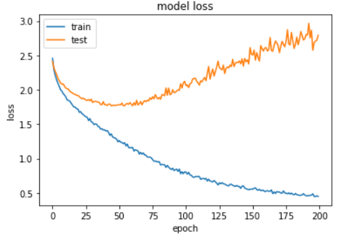
Visual training results:
plt.plot(history.history['loss'])
plt.plot(history.history['val_loss'])
plt.title('model loss')
plt.ylabel('loss')
plt.xlabel('epoch')
plt.legend(['train', 'test'], loc='upper left')
plt.show()
plt.plot(history.history['acc'])
plt.plot(history.history['val_acc'])
plt.title('model acc')
plt.ylabel('acc')
plt.xlabel('epoch')
plt.legend(['train', 'test'], loc='upper left')
plt.show()
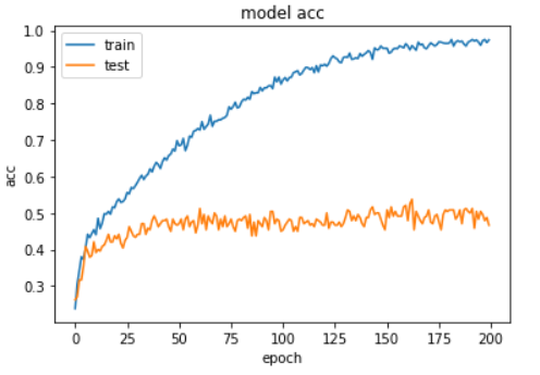
It can be seen from the above figure that the model starts to be fitted after 60 rounds of training, at this time, the training accuracy reaches 70%, and the verification accuracy reaches 50%. After 200 rounds of training, the training accuracy reaches 95%.
test
Finally, the trained model is tested.
from keras.models import load_model
import pickle

model=load_model('speech_mfcc_model.h5')
paradict={}
with open('mfcc_model_para_dict.pkl', 'rb') as f:
    paradict=pickle.load(f)
DATA_MEAN=paradict['mean']
DATA_STD=paradict['std']
emotionDict=paradict['emotion']
edr = dict([(i, t) for t, i in emotionDict.items()])

import librosa

filePath=r'record1.wav'
y,sr = librosa.load(filePath,sr=None)
y=normalizeVoiceLen(y,VOICE_LEN)#Normalized length
mfcc_data=librosa.feature.mfcc(y=y, sr=sr,n_mfcc=13,n_fft=N_FFT,hop_length=int(N_FFT/4))
feature=np.mean(mfcc_data,axis=0)
feature=feature.reshape((126,1))
feature-=DATA_MEAN
feature/=DATA_STD
feature=feature.reshape((1,126,1))
result=model.predict(feature)
index=np.argmax(result, axis=1)[0]
print(edr[index])
Let's share, grow together, and share so that we are not alone in programming. Scan the QR code quickly and study happily with the blogger!