1. Introduction to Sparse Representation

1 Sparse Representation Theory
Sparse means that most or all of the original signals are represented by a linear combination of fewer basic signals. After sparse representation, the more sparse the signal is, the more accurate the reconstructed signal will be. Set x< Rn as the signal to be processed and D< Rn*m as the dictionary, then x can be represented as:

In the formula: _ < Rm, _= (theta 1, theta 2..., theta m) is the sparsity factor;D(n_m) is an over-complete dictionary. Formula (1) can be derived from Formula (2) by adding the sparsity constraint:

Formula 0 denotes the l0 norm, which denotes the number of non-zero elements in. The exact sparse representation of Formula (2) is usually unsatisfactory and its approximation can be described as:

v < Rn is an approximation error, so equation (2) is converted to solution of equation (3).

The direct solution of the l0 norm is a NP-hard problem for which either a relaxation algorithm or a greedy algorithm can be used.
The sparse decomposition algorithm in sparse representation was first proposed by Mallat. The Matching Pursuit (MP) algorithm proposed by Mallat is simple and easy to implement, so it has been widely used. Subsequently, researchers have proposed improved algorithms based on MP algorithm, such as Orthogonal Matching Pursuit (OMP), which converges faster than MP algorithm.

2 Multispectral image fusion based on sparse representation
This paper presents a multispectral image fusion method based on sparse representation, which is implemented as follows:
Step1: The multispectral image is transformed by PCA to get the first principal component of the image.
Step2: Match the histogram with the panchromatic image and the first principal component;
Step3: The first principal component and the matched panchromatic image are divided into blocks, each image block is represented sparsely, and the sparse coefficients are fused using absolute maximization.
Step4: The fusion coefficient is reconstructed to obtain the fused multispectral image.

2. Partial Source Code

%%%%%%%%%%%%%%%%%%%%%%%%%%%%%%%%%%%%%%%%%%%%%%%%%%%%%%%%%%%%%%%%%%%%%%%%%%%%%%%%%%%%%%%%%%%%%%%%%
%%  The implementation of Hybrid Monte Carlo method to evaluate the joint posterior distribution
%   AUTHOR: Qi WEI, University of Toulouse, qi.wei@n7.fr
%%%%%%%%%%%%%%%%%%%%%%%%%%%%%%%%%%%%%%%%%%%%%%%%%%%%%%%%%%%%%%%%%%%%%%%%%%%%%%%%%%%%%%%%%%%%%%%%%
close all;clear all;
setup;
Verbose='on';
generate=1;subMeth='PCA';FusMeth='Sparse';
scale=1;SNR_R=inf;seed=1;
%% Generate the data
[name_image,band_remove,band_set,nr,nc,N_band,nb_sub,X_real,XH,XHd,XHd_int,XM,VXH,VXM,psfY,psfZ_unk,...
    sigma2y_real,sigma2z_real,SNR_HS,SNR_MS,miu_x_real,s2_real,P_inc,P_dec,eig_val]=Para_Set(seed,scale,subMeth,SNR_R);
%%%%%%%%%%%%%%%%%%%%%%%%%%%%%%%%%%%%%%%%%%%%%%%%%%%%%%%%%%%%%%%%%%%%%%%%%%%%%%%%%%%%%%%%%%%%%%%%%%%
%Sparse fusion consists three parts
%%%%%%%%%%%%%%%%%%%%%%%%%%%%%%%%%%%%%%%%%%%%%%%%%%%%%%%%%%%%%%%%%%%%%%%%%%%%%%%%%%%%%%%%%%%%%%%%%%%
%% Step 1: Learn the rough estimation
learn_dic=1;train_support=1;Para_Prior_Initial;
X_source=RoughEst(XM,XH,XHd,psfY,nb_sub,P_dec);
%% Step 2: Learn the dictionary
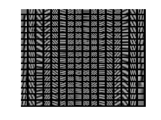
[time_LD,Dic,supp]=Dic_Para(X_source,P_inc,learn_dic,train_support,X_real,0);
%% Step 3: Alternating optimization
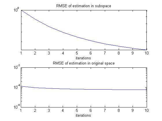
[HSFusion.(FusMeth),Costime,diff_X,RMSE_sub,RMSE_org,tau_d_set,VXd_dec]=AlterOpti(X_source,XH,XM,psfY,...
    psfZ_unk,sigma2y_real,sigma2z_real,P_dec,P_inc,FusMeth,X_real,Dic,supp);
%% Evaluate the fusion results: Quantitative
[err_max.(FusMeth),err_l1.(FusMeth),err_l2.(FusMeth),SNR.(FusMeth),Q.(FusMeth),SAM_m.(FusMeth),RMSE_fusion.(FusMeth),...
    ERGAS.(FusMeth),DD.(FusMeth)] = metrics(X_real,HSFusion.(FusMeth),psfY.ds_r);
fprintf('%s Performance:\n SNR: %f\n RMSE: %f\n UIQI: %f\n SAM: %f\n ERGAS: %f\n DD: %f\n Time: %f\n',...
    FusMeth,SNR.(FusMeth),RMSE_fusion.(FusMeth),Q.(FusMeth),SAM_m.(FusMeth),ERGAS.(FusMeth),DD.(FusMeth),Costime.(FusMeth));
%% Display the fusion results: Qualitive
normColor = @(R)max(min((R-mean(R(:)))/std(R(:)),2),-2)/3+0.5;
temp_show=X_real(:,:,band_set);temp_show=normColor(temp_show);
figure(113);imshow(temp_show);title('Groundtruth')
temp_show=XHd_int(:,:,band_set);temp_show=normColor(temp_show);
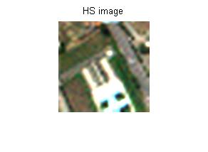
figure(114);imshow(temp_show);title('HS image')
temp_show=mean(XM,3);temp_show=normColor(temp_show);
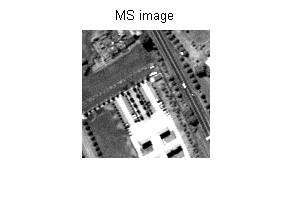
figure(115);imshow(temp_show);title('MS image')
temp_show=HSFusion.(FusMeth)(:,:,band_set);temp_show=normColor(temp_show);
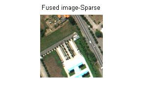
figure(116);imshow(temp_show);title(['Fused image-' FusMeth])
name=[mat2str(clock) FusMeth '.mat'];save(name);

3

3. Operation results

4. matlab Versions and References

1 matlab version
2014a

2 References
[1] Cai Limei. MATLAB Image Processing - Theory, Algorithm and Example Analysis [M]. Tsinghua University Press, 2020.
[2] Yang Dan, Zhao Haibin, Longzhe.MATLAB image processing example in detail [M]. Tsinghua University Press, 2013.
[3] Zhou Pin. MATLAB Image Processing and Graphical User Interface Design [M]. Tsinghua University Press, 2013.
[4] Liu Chenglong. Proficient in MATLAB image processing [M]. Tsinghua University Press, 2015.