The article was originally written in Mars team column , welcome to follow.
From this article, we start a new series of reading paper.
Today's paper is Towards Scalable Dataframe Systems , is still a preprint. By Devin Petersohn from Riselab , formerly known as APMLab, the lab has produced a series of famous open source projects, such as Apache Spark, Apache Mesos, etc.
Personally, I think this paper is quite meaningful. For the first time (as far as I know), I tried to define DataFrame academically, which gave a good theoretical guidance.
This article I will not stick to the original paper, I will add my own understanding. This article will be roughly divided into three parts:
- What is a real DataFrame?
- Why is the so-called DataFrame system, such as Spark DataFrame, killing the original meaning of DataFrame.
- Look at this from the perspective of Mars DataFrame.
What is a real DataFrame?
origin
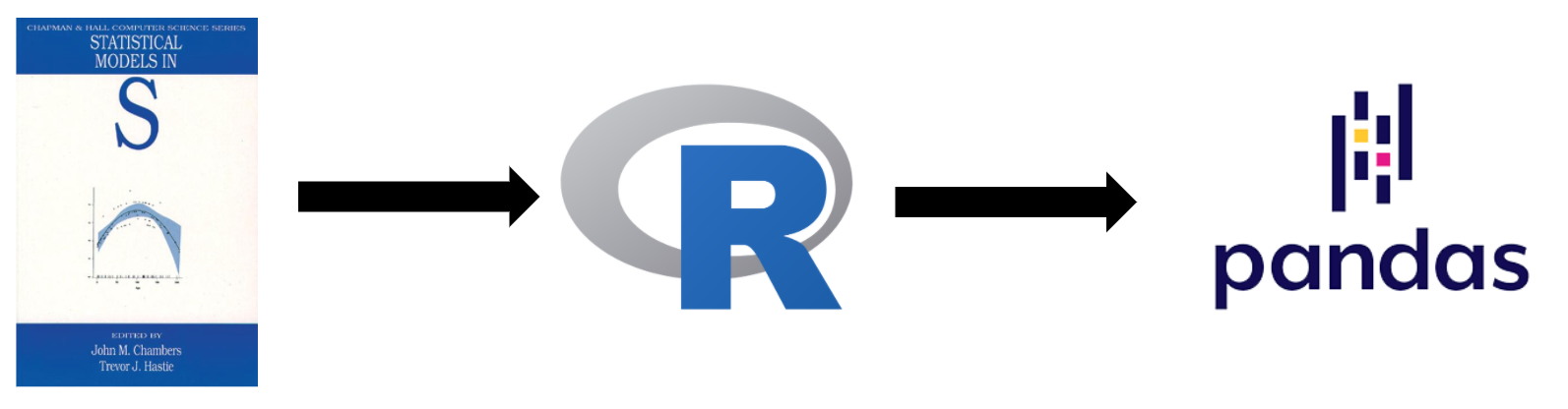
The earliest "data frame" (initially known as "data frame") originated from the S language developed by Bell Labs. The "data frame" was published in 1990. Chapter 3 of the book "S language statistical model" details its concept and emphasizes the origin of the matrix of the data frame.
The data frame described in the book looks like a matrix, and supports matrix like operations; at the same time, it looks like a relational table.
R language, as an open source version of S language, released the first stable version in 2000, and implemented dataframe. pandas It was developed in 2009, and the concept of DataFrame came into Python. These dataframes are of the same origin and have the same semantics and data model.
DataFrame data model
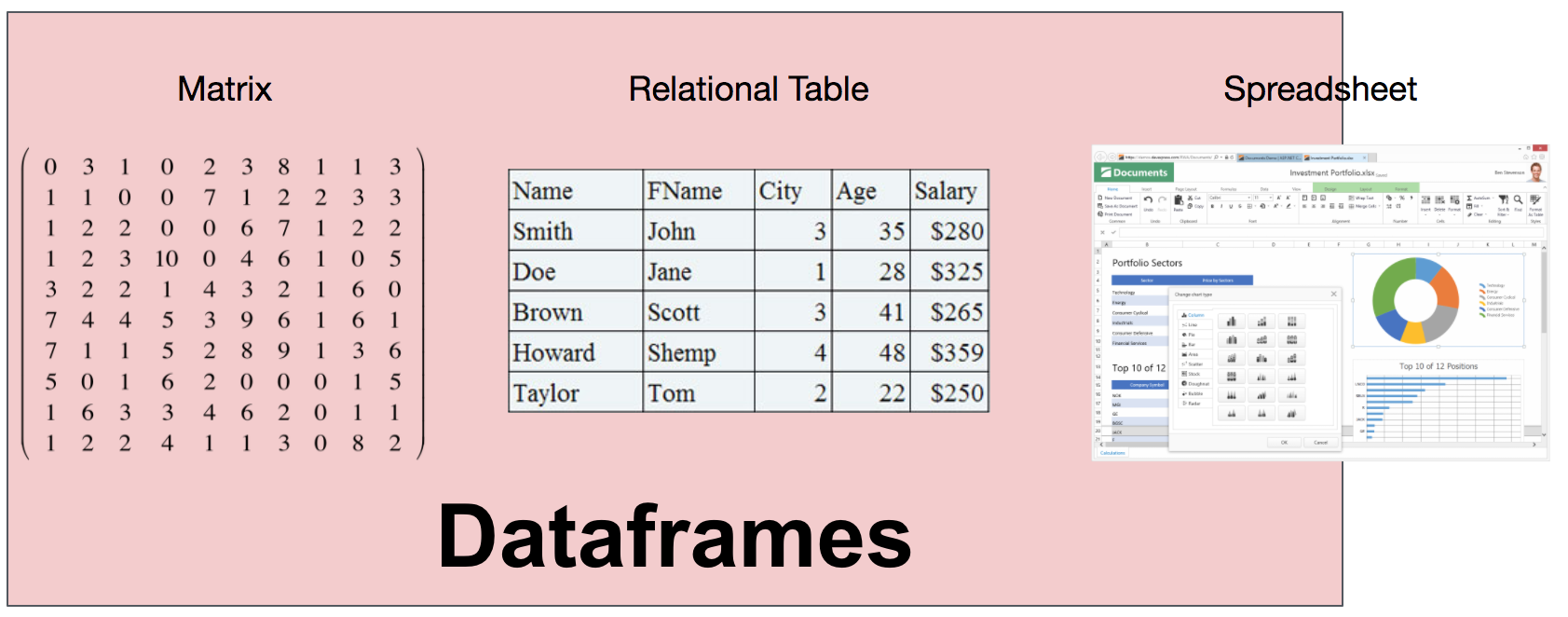
The need for DataFrame comes from seeing data as matrices and tables. However, there is only one data type in the matrix, which is too limited; at the same time, relational tables require that data must first define schema. For DataFrame, its column type can be inferred at run time, without knowing in advance or requiring all columns to be of the same type. Therefore, DataFrame can be understood as a combination of relational systems, matrices, and even spreadsheet programs (typically Excel).
Compared with relational systems, DataFrame has several interesting properties, which makes it unique.
Ensure sequence, row and column symmetry
First, no matter in the direction of row or column, DataFrame has order; and row and column are first-class citizens, so they will not be treated differently.
Take pandas for example. When a DataFrame is created, the data on both rows and columns are in order. Therefore, you can use positions to select data on both rows and columns.
In [1]: import pandas as pd

In [2]: import numpy as np

In [3]: df = pd.DataFrame(np.random.rand(5, 4))

In [4]: df
Out[4]:
          0         1         2         3
0  0.736385  0.271232  0.940270  0.926548
1  0.319533  0.891928  0.471176  0.583895
2  0.440825  0.500724  0.402782  0.109702
3  0.300279  0.483571  0.639299  0.778849
4  0.341113  0.813870  0.054731  0.059262

In [5]: df.at[2, 2]  # Second row second column element
Out[5]: 0.40278182653648853
Because of the symmetry between rows and columns, aggregate functions can be calculated in both directions, just specify axis.
In [6]: df.sum()  # Default axis == 0, aggregate in row direction, so the result is 4 elements
Out[6]:
0    2.138135
1    2.961325
2    2.508257
3    2.458257
dtype: float64

In [7]: df.sum(axis=1)  # axis == 1, aggregate in column direction, so it is 5 elements
Out[7]:
0    2.874434
1    2.266533
2    1.454032
3    2.201998
4    1.268976
dtype: float64
If you are familiar with numpy (numerical calculation library, including the definition of multidimensional array and matrix), you can see that this feature is very familiar, so you can see the matrix essence of DataFrame.
Rich API
The API of DataFrame is very rich, covering relationships (such as filter, join), linear algebra (such as post, dot) and operations like spreadsheets (such as pivot).
Take pandas for example. A DataFrame can be transposed to make rows and columns swap.
In [8]: df.transpose()
Out[8]:
          0         1         2         3         4
0  0.736385  0.319533  0.440825  0.300279  0.341113
1  0.271232  0.891928  0.500724  0.483571  0.813870
2  0.940270  0.471176  0.402782  0.639299  0.054731
3  0.926548  0.583895  0.109702  0.778849  0.059262
Intuitive syntax for interactive analysis
Users can continuously explore the data of DataFrame, query results can be reused by subsequent results, and it is very convenient to combine very complex operations in the way of programming, which is very suitable for interactive analysis.
Allow heterogeneous data in columns
DataFrame's type system allows the existence of heterogeneous data in a column. For example, an int column allows the existence of string type data, which may be dirty data. This shows that DataFrame is very flexible.
In [10]: df2 = df.copy()

In [11]: df2.iloc[0, 0] = 'a'

In [12]: df2
Out[12]:
          0         1         2         3
0         a  0.271232  0.940270  0.926548
1  0.319533  0.891928  0.471176  0.583895
2  0.440825  0.500724  0.402782  0.109702
3  0.300279  0.483571  0.639299  0.778849
4  0.341113  0.813870  0.054731  0.059262
data model
Now we can formally define what a real DataFrame is:
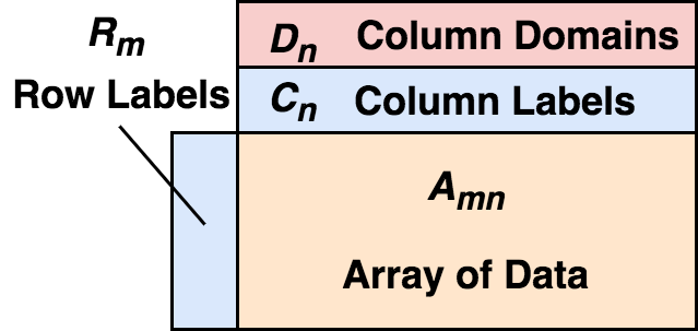
DataFrame consists of two-dimensional mixed type arrays, row labels, column labels, and types (types or domains). On each column, this type is optional and can be inferred at run time. From the perspective of rows, DataFrame can be seen as the mapping from row label to row, and the order between rows can be guaranteed; from the perspective of columns, it can be seen as the mapping from column type to column label to column, as well as the order between columns.
The existence of row label and column label makes it very convenient to select data.
In [13]: df.index = pd.date_range('2020-4-15', periods=5)

In [14]: df.columns = ['c1', 'c2', 'c3', 'c4']

In [15]: df
Out[15]:
                  c1        c2        c3        c4
2020-04-15  0.736385  0.271232  0.940270  0.926548
2020-04-16  0.319533  0.891928  0.471176  0.583895
2020-04-17  0.440825  0.500724  0.402782  0.109702
2020-04-18  0.300279  0.483571  0.639299  0.778849
2020-04-19  0.341113  0.813870  0.054731  0.059262

In [16]: df.loc['2020-4-16': '2020-4-18', 'c2': 'c3']  # Notice that the slice here is a closed interval
Out[16]:
                  c2        c3
2020-04-16  0.891928  0.471176
2020-04-17  0.500724  0.402782
2020-04-18  0.483571  0.639299
Here, index and columns are row and column labels respectively. We can easily select a period of time (select on row) and several columns (select on column) of data. Of course, these are based on the sequential storage of data.
The sequential storage feature makes DataFrame very suitable for statistical work.
In [17]: df3 = df.shift(1)  # Move the data of df down one grid and keep the row column index unchanged

In [18]: df3
Out[18]:
                  c1        c2        c3        c4
2020-04-15       NaN       NaN       NaN       NaN
2020-04-16  0.736385  0.271232  0.940270  0.926548
2020-04-17  0.319533  0.891928  0.471176  0.583895
2020-04-18  0.440825  0.500724  0.402782  0.109702
2020-04-19  0.300279  0.483571  0.639299  0.778849

In [19]: df - df3  # Data subtraction is automatically aligned by label, so this step can be used to calculate the aspect ratio
Out[19]:
                  c1        c2        c3        c4
2020-04-15       NaN       NaN       NaN       NaN
2020-04-16 -0.416852  0.620697 -0.469093 -0.342653
2020-04-17  0.121293 -0.391205 -0.068395 -0.474194
2020-04-18 -0.140546 -0.017152  0.236517  0.669148
2020-04-19  0.040834  0.330299 -0.584568 -0.719587

In [21]: (df - df3).bfill()  # Empty data in the first row is filled in the next row
Out[21]:
                  c1        c2        c3        c4
2020-04-15 -0.416852  0.620697 -0.469093 -0.342653
2020-04-16 -0.416852  0.620697 -0.469093 -0.342653
2020-04-17  0.121293 -0.391205 -0.068395 -0.474194
2020-04-18 -0.140546 -0.017152  0.236517  0.669148
2020-04-19  0.040834  0.330299 -0.584568 -0.719587
From the example, we can see that just because the data is stored in order, we can keep the index unchanged and move down one row as a whole, so that yesterday's data is on today's row, and then take the original data minus the displaced data, because the DataFrame It will automatically align by label, so for a date, it is equivalent to subtracting the data of the previous day from the data of the current day, so you can do the operation similar to the ring comparison. It's just too convenient. Imagine, for a relational system, I'm afraid we need to find a list of join conditions, and then do subtraction and so on. Finally, for empty data, we can also fill in the data of the previous row (fill) or the next row (bfill). It takes a lot of work to achieve the same effect in a relationship system.
The real meaning of DataFrame is being killed
In recent years, DataFrame systems have mushroomed. However, most of these systems only contain the semantics of relational tables, not the meaning of matrices as we said before, and most of them do not guarantee the order of data. Therefore, the characteristics of statistics and machine learning that real DataFrame possesses no longer exist. These "DataFrame" systems make the word "DataFrame" almost meaningless. In order to deal with large-scale data, data scientists have to change their way of thinking, which inevitably involves risks.
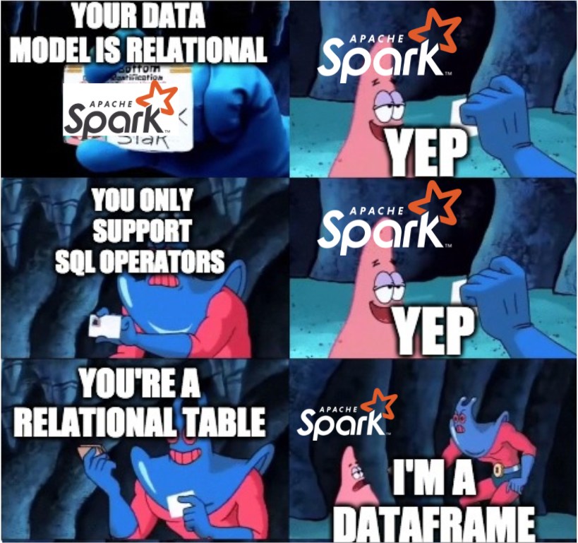
Spark DataFrame and Koalas are not real dataframes
The representative of these DataFrame systems is spark DataFrame. Spark is great, of course. It solves the problem of data scale. At the same time, it brings the concept of "DataFrame" to the field of big data for the first time. But in fact, it is just another form of spark.sql (of course, spark DataFrame is under spark.sql). Spark DataFrame only contains the semantics of relational tables, the schema needs to be determined, and the data does not guarantee the order.
Then some students will say Koalas What about it? Koalas provides the pandas API, which can be analyzed on spark with the syntax of pandas. In fact, because koalas also transfers the operations of pandas to the Spark DataFrame for execution, because of the features of the Spark DataFrame kernel itself, koalas is doomed to only look the same as pandas.
To illustrate this, we use data set(Hourly Ridership by Origin-Destination Pairs ), only data in 2019 will be taken.
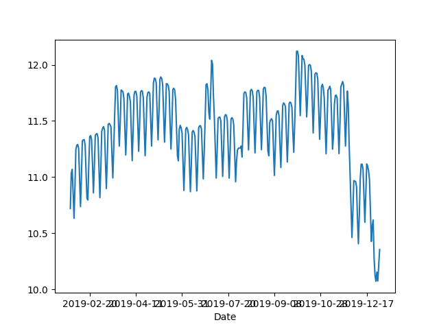
For pandas, we aggregate by day and average by sliding the window for 30 days.
In [22]: df = pd.read_csv('Downloads/bart-dataset/date-hour-soo-dest-2019.csv',
    ...: names=['Date','Hour','Origin','Destination','Trip Count'])

In [23]: df.groupby('Date').mean()['Trip Count'].rolling(30).mean().plot()
Out[23]: <matplotlib.axes._subplots.AxesSubplot at 0x118077d90>
If it's Koalas, because its API looks the same as panda's, we will replace it with import according to Koalas's documents.
In [1]: import databricks.koalas as ks

In [2]: df = ks.read_csv('Downloads/bart-dataset/date-hour-soo-dest-2019.csv', names=['Date','Hour','Origin','Destination','Trip Count'])

In [3]: df.groupby('Date').mean()['Trip Count'].rolling(30).mean().plot()
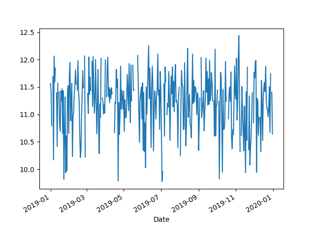
Then surprisingly, the results were not consistent. It took a long time to find out. The reason is the order problem. Sorting is not guaranteed after aggregation results. Therefore, to get the same results, you need to add sort_index() before rolling to ensure that the results after groupby are sorted.
In [4]: df.groupby('Date').mean()['Trip Count'].sort_index().rolling(30).mean().plot()
The default collation is very important, especially for data indexed by time, and it makes it easier for data scientists to observe data and reproduce results.
Therefore, when using Koalas, please be careful and always pay attention to whether your data is sorted in your mind, because Koalas may not behave as you think.
Let's look at shift again. One premise that it can work is that data is sorted. What happens in Koalas?
In [6]: df.shift(1)
---------------------------------------------------------------------------
Py4JJavaError                             Traceback (most recent call last)
/usr/local/opt/apache-spark/libexec/python/pyspark/sql/utils.py in deco(*a, **kw)
     62         try:
---> 63             return f(*a, **kw)
     64         except py4j.protocol.Py4JJavaError as e:

/usr/local/opt/apache-spark/libexec/python/lib/py4j-0.10.7-src.zip/py4j/protocol.py in get_return_value(answer, gateway_client, target_id, name)
    327                     "An error occurred while calling {0}{1}{2}.\n".
--> 328                     format(target_id, ".", name), value)
    329             else:

Py4JJavaError: An error occurred while calling o110.select.
: org.apache.spark.sql.AnalysisException: cannot resolve 'isnan(lag(`Date`, 1, NULL) OVER (ORDER BY `__natural_order__` ASC NULLS FIRST ROWS BETWEEN -1 FOLLOWING AND -1 FOLLOWING))' due to data type mismatch: argument 1 requires (double or float) type, however, 'lag(`Date`, 1, NULL) OVER (ORDER BY `__natural_order__` ASC NULLS FIRST ROWS BETWEEN -1 FOLLOWING AND -1 FOLLOWING)' is of timestamp type.;;
'Project [__index_level_0__#41, CASE WHEN (isnull(lag(Date#30, 1, null) windowspecdefinition(__natural_order__#50L ASC NULLS FIRST, specifiedwindowframe(RowFrame, -1, -1))) || isnan(lag(Date#30, 1, null) windowspecdefinition(__natural_order__#50L ASC NULLS FIRST, specifiedwindowframe(RowFrame, -1, -1)))) THEN null ELSE lag(Date#30, 1, null) windowspecdefinition(__natural_order__#50L ASC NULLS FIRST, specifiedwindowframe(RowFrame, -1, -1)) END AS Date#87, CASE WHEN (isnull(lag(Hour#31, 1, null) windowspecdefinition(__natural_order__#50L ASC NULLS FIRST, specifiedwindowframe(RowFrame, -1, -1))) || isnan(cast(lag(Hour#31, 1, null) windowspecdefinition(__natural_order__#50L ASC NULLS FIRST, specifiedwindowframe(RowFrame, -1, -1)) as double))) THEN cast(null as int) ELSE lag(Hour#31, 1, null) windowspecdefinition(__natural_order__#50L ASC NULLS FIRST, specifiedwindowframe(RowFrame, -1, -1)) END AS Hour#88, CASE WHEN (isnull(lag(Origin#32, 1, null) windowspecdefinition(__natural_order__#50L ASC NULLS FIRST, specifiedwindowframe(RowFrame, -1, -1))) || isnan(cast(lag(Origin#32, 1, null) windowspecdefinition(__natural_order__#50L ASC NULLS FIRST, specifiedwindowframe(RowFrame, -1, -1)) as double))) THEN cast(null as string) ELSE lag(Origin#32, 1, null) windowspecdefinition(__natural_order__#50L ASC NULLS FIRST, specifiedwindowframe(RowFrame, -1, -1)) END AS Origin#89, CASE WHEN (isnull(lag(Destination#33, 1, null) windowspecdefinition(__natural_order__#50L ASC NULLS FIRST, specifiedwindowframe(RowFrame, -1, -1))) || isnan(cast(lag(Destination#33, 1, null) windowspecdefinition(__natural_order__#50L ASC NULLS FIRST, specifiedwindowframe(RowFrame, -1, -1)) as double))) THEN cast(null as string) ELSE lag(Destination#33, 1, null) windowspecdefinition(__natural_order__#50L ASC NULLS FIRST, specifiedwindowframe(RowFrame, -1, -1)) END AS Destination#90, CASE WHEN (isnull(lag(Trip Count#34, 1, null) windowspecdefinition(__natural_order__#50L ASC NULLS FIRST, specifiedwindowframe(RowFrame, -1, -1))) || isnan(cast(lag(Trip Count#34, 1, null) windowspecdefinition(__natural_order__#50L ASC NULLS FIRST, specifiedwindowframe(RowFrame, -1, -1)) as double))) THEN cast(null as int) ELSE lag(Trip Count#34, 1, null) windowspecdefinition(__natural_order__#50L ASC NULLS FIRST, specifiedwindowframe(RowFrame, -1, -1)) END AS Trip Count#91, __natural_order__#50L]
+- Project [__index_level_0__#41, Date#30, Hour#31, Origin#32, Destination#33, Trip Count#34, monotonically_increasing_id() AS __natural_order__#50L]
   +- Project [__index_level_0__#41, Date#30, Hour#31, Origin#32, Destination#33, Trip Count#34]
      +- Project [Date#30, Hour#31, Origin#32, Destination#33, Trip Count#34, _w0#42L, _we0#43, (_we0#43 - 1) AS __index_level_0__#41]
         +- Window [row_number() windowspecdefinition(_w0#42L ASC NULLS FIRST, specifiedwindowframe(RowFrame, unboundedpreceding$(), currentrow$())) AS _we0#43], [_w0#42L ASC NULLS FIRST]
            +- Project [Date#30, Hour#31, Origin#32, Destination#33, Trip Count#34, monotonically_increasing_id() AS _w0#42L]
               +- Project [0#20 AS Date#30, 1#21 AS Hour#31, 2#22 AS Origin#32, 3#23 AS Destination#33, 4#24 AS Trip Count#34]
                  +- Project [_c0#10 AS 0#20, _c1#11 AS 1#21, _c2#12 AS 2#22, _c3#13 AS 3#23, _c4#14 AS 4#24]
                     +- Relation[_c0#10,_c1#11,_c2#12,_c3#13,_c4#14] csv

    at org.apache.spark.sql.catalyst.analysis.package$AnalysisErrorAt.failAnalysis(package.scala:42)
    at org.apache.spark.sql.catalyst.analysis.CheckAnalysis$$anonfun$checkAnalysis$1$$anonfun$apply$3.applyOrElse(CheckAnalysis.scala:116)
    at org.apache.spark.sql.catalyst.analysis.CheckAnalysis$$anonfun$checkAnalysis$1$$anonfun$apply$3.applyOrElse(CheckAnalysis.scala:108)
    at org.apache.spark.sql.catalyst.trees.TreeNode$$anonfun$transformUp$1.apply(TreeNode.scala:280)
    at org.apache.spark.sql.catalyst.trees.TreeNode$$anonfun$transformUp$1.apply(TreeNode.scala:280)
    at org.apache.spark.sql.catalyst.trees.CurrentOrigin$.withOrigin(TreeNode.scala:69)
    at org.apache.spark.sql.catalyst.trees.TreeNode.transformUp(TreeNode.scala:279)
    at org.apache.spark.sql.catalyst.trees.TreeNode$$anonfun$3.apply(TreeNode.scala:277)
    at org.apache.spark.sql.catalyst.trees.TreeNode$$anonfun$3.apply(TreeNode.scala:277)
    at org.apache.spark.sql.catalyst.trees.TreeNode$$anonfun$4.apply(TreeNode.scala:328)
    at org.apache.spark.sql.catalyst.trees.TreeNode.mapProductIterator(TreeNode.scala:186)
    at org.apache.spark.sql.catalyst.trees.TreeNode.mapChildren(TreeNode.scala:326)
    at org.apache.spark.sql.catalyst.trees.TreeNode.transformUp(TreeNode.scala:277)
    at org.apache.spark.sql.catalyst.trees.TreeNode$$anonfun$3.apply(TreeNode.scala:277)
    at org.apache.spark.sql.catalyst.trees.TreeNode$$anonfun$3.apply(TreeNode.scala:277)
    at org.apache.spark.sql.catalyst.trees.TreeNode.org$apache$spark$sql$catalyst$trees$TreeNode$$mapChild$2(TreeNode.scala:306)
    at org.apache.spark.sql.catalyst.trees.TreeNode$$anonfun$4$$anonfun$apply$13.apply(TreeNode.scala:356)
    at scala.collection.TraversableLike$$anonfun$map$1.apply(TraversableLike.scala:234)
    at scala.collection.TraversableLike$$anonfun$map$1.apply(TraversableLike.scala:234)
    at scala.collection.immutable.List.foreach(List.scala:392)
    at scala.collection.TraversableLike$class.map(TraversableLike.scala:234)
    at scala.collection.immutable.List.map(List.scala:296)
    at org.apache.spark.sql.catalyst.trees.TreeNode$$anonfun$4.apply(TreeNode.scala:356)
    at org.apache.spark.sql.catalyst.trees.TreeNode.mapProductIterator(TreeNode.scala:186)
    at org.apache.spark.sql.catalyst.trees.TreeNode.mapChildren(TreeNode.scala:326)
    at org.apache.spark.sql.catalyst.trees.TreeNode.transformUp(TreeNode.scala:277)
    at org.apache.spark.sql.catalyst.trees.TreeNode$$anonfun$3.apply(TreeNode.scala:277)
    at org.apache.spark.sql.catalyst.trees.TreeNode$$anonfun$3.apply(TreeNode.scala:277)
    at org.apache.spark.sql.catalyst.trees.TreeNode$$anonfun$4.apply(TreeNode.scala:328)
    at org.apache.spark.sql.catalyst.trees.TreeNode.mapProductIterator(TreeNode.scala:186)
    at org.apache.spark.sql.catalyst.trees.TreeNode.mapChildren(TreeNode.scala:326)
    at org.apache.spark.sql.catalyst.trees.TreeNode.transformUp(TreeNode.scala:277)
    at
  ...  # There is also a large section of error information, which is omitted here
This error report may shock the data scientists. Whatever, I made a shift. The error report is mixed with Java exception stack and a lot of unreadable errors.
The real error here is related to the fact that Date is a time stamp, so we can only take the field of int type as shift.
In [10]: df['Hour'].shift(1)
Out[10]: 20/04/20 17:22:38 WARN WindowExec: No Partition Defined for Window operation! Moving all data to a single partition, this can cause serious performance degradation.
20/04/20 17:22:38 WARN WindowExec: No Partition Defined for Window operation! Moving all data to a single partition, this can cause serious performance degradation.
It can run, but I see a sentence to the effect that the data will be put into a partition for execution. This is precisely because the data itself does not guarantee the order, so we can only collect the data together, sort it, and then call shift. This is no longer a distributed program, even slower than pandas itself.
Matrix related operations such as DataFrame.dot are also not included in Koalas, which are difficult to express in relation algebra.
PyODPS DataFrame
I believe I have used MaxCompute (formerly ODPS, Alibaba cloud's self-developed big data system), and I should have heard of PyODPS. This library is a product of our previous years. A DataFrame is also included in PyODPS, and PyODPS DataFrame will be compiled to ODPS SQL for execution.
The reason for mentioning PyODPS DataFrame is that we found a few years ago that although it provides the pandas like interface, to some extent, it enables users to solve problems with pandas like thinking. However, when users ask us, how to fill in data backward? How to get data through index? The answer is No. The reason is the same, because PyODPS DataFrame only proxy the calculation to the engine that does not guarantee the order and only relational algebra operators.
If the data model of the system itself is not the real data frame model, it is not enough to just make the interface look like it.
Mars DataFrame
So when it comes to Mars DataFrame, we actually do Mars The original intention is consistent with the paper's idea, because although the existing system can solve the scale problem well, the good parts of the traditional data science package are really forgotten. We hope Mars can keep the good parts of these libraries, solve the scale problem, and make full use of the new hardware.
Mars DataFrame will automatically split the DataFrame into many small chunks. Each chunk is also a DataFrame, and the data between chunks or within chunks is in order.
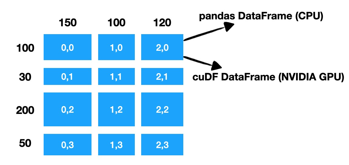
In the example in the figure, a DataFrame with 380 rows and 370 columns is divided into 9 chunk s by Mars. According to whether the calculation is on CPU or NVIDIA GPU, use panda DataFrame or cuDF DataFrame to store data and perform real calculations. As you can see, Mars will split on both rows and columns. This kind of equivalence on rows and columns makes the matrix nature of DataFrame play a role.
When a single machine actually executes, Mars will automatically distribute the data to multi-core or multi card execution according to the location of the initial data; for distributed, it will distribute the calculation to multiple machines for execution.
Mars DataFrame retains the concepts of row labels, column labels, and types. Therefore, it can be imagined that, like pandas, you can filter according to the tags on a relatively large data set.
In [1]: import mars.dataframe as md

In [2]: import mars.tensor as mt

In [8]: df = md.DataFrame(mt.random.rand(10000, 10, chunk_size=1000),
   ...:                   index=md.date_range('2020-1-1', periods=10000))

In [9]: df.loc['2020-4-15'].execute()
Out[9]:
0    0.622763
1    0.446635
2    0.007870
3    0.107846
4    0.288893
5    0.219340
6    0.228806
7    0.969435
8    0.033130
9    0.853619
Name: 2020-04-15 00:00:00, dtype: float64
Mars will maintain the same sorting characteristics as pandas, so for operations such as groupby, you don't need to worry about the inconsistency between the results and what you want.
In [6]: import mars.dataframe as md

In [7]: df = md.read_csv('Downloads/bart-dataset/date-hour-soo-dest-2019.csv', n
   ...: ames=['Date','Hour','Origin','Destination','Trip Count'])

In [8]: df.groupby('Date').mean()['Trip Count'].rolling(30).mean().plot() # The results are correct
Out[8]: <matplotlib.axes._subplots.AxesSubplot at 0x11ff8ab90>
For shift, not only the result is correct, but also the ability of multi-core, multi card and distributed can be utilized during execution.
In [3]: df.shift(1).head(10).execute()
Out[3]:
         Date  Hour Origin Destination  Trip Count
0         NaN   NaN    NaN         NaN         NaN
1  2019-01-01   0.0   12TH        16TH         4.0
2  2019-01-01   0.0   12TH        ANTC         1.0
3  2019-01-01   0.0   12TH        BAYF         1.0
4  2019-01-01   0.0   12TH        CIVC         2.0
5  2019-01-01   0.0   12TH        COLM         1.0
6  2019-01-01   0.0   12TH        COLS         1.0
7  2019-01-01   0.0   12TH        CONC         1.0
8  2019-01-01   0.0   12TH        DALY         1.0
9  2019-01-01   0.0   12TH        DELN         2.0
Not just DataFrame
Mars also includes the sensor module to support parallel and distributed numpy, and the learn module to parallel and distributed scik it learn, so it can be imagined that for example, mars.sensor.linkage.svd can directly act on Mars DataFrame, which gives Mars semantics beyond DataFrame itself.
In [1]: import mars.dataframe as md

In [2]: import mars.tensor as mt

In [3]: df = md.DataFrame(mt.random.rand(10000, 10, chunk_size=1000))

In [5]: mt.linalg.svd(df).execute()
summary
"Towards Scalable DataFrame Systems" gives the academic definition of DataFrame. In order to be extensible, the first is the real DataFrame, and the second is extensible.
In our opinion, Mars It's a real DataFrame. It's born to be extensible, and Mars isn't just a DataFrame. In our view, Mars has great potential in the field of data science.
Mars was born in MaxCompute team. MaxCompute, formerly ODPS, is a fast and fully hosted EB level data warehouse solution. Mars is about to provide services through MaxCompute. Users who have purchased MaxCompute services will be able to experience Mars services out of the box. Coming soon.
Reference resources
- Towards Scalable Dataframe Systems: https://arxiv.org/abs/2001.00888
- Preventing the Death of the DataFrame: https://towardsdatascience.com/preventing-the-death-of-the-dataframe-8bca1c0f83c8
If you're interested in Mars, you can follow Mars team column , or nail scan QR code to join Mars discussion group.