1, Naive Bayes overview

Naive Bayesian method is a classification method based on Bayesian theorem and the assumption of feature conditional independence. For a given training set, firstly, the joint probability distribution of input and output is learned based on the independent assumption of characteristic conditions (the naive Bayes method, which obtains the model through learning, obviously belongs to the generative model); Then, based on this model, for a given input x, the output y with the maximum a posteriori probability is obtained by using Bayesian theorem

2, Basic formula of naive Bayes

1. Joint distribution rate

The joint probability is expressed as the probability that multiple conditions are included and all conditions are true at the same time, which is recorded as P (x = a, y = b) P (x = a, y = b) P (x = a, y = b) or P (a, b) P (a, b) or P (a, b) P (AB) P (AB)

2. Conditional probability

There is a jar containing 7 stones, of which 3 are white and 4 are black. If a stone is taken randomly from the jar, what is the probability that it is a white stone

Obviously, the probability of taking out white stone is 3 / 7 and the probability of taking out black stone is 4 / 7. We use   P(white)   The probability value can be obtained by dividing the number of white stones by the total number of stones.  

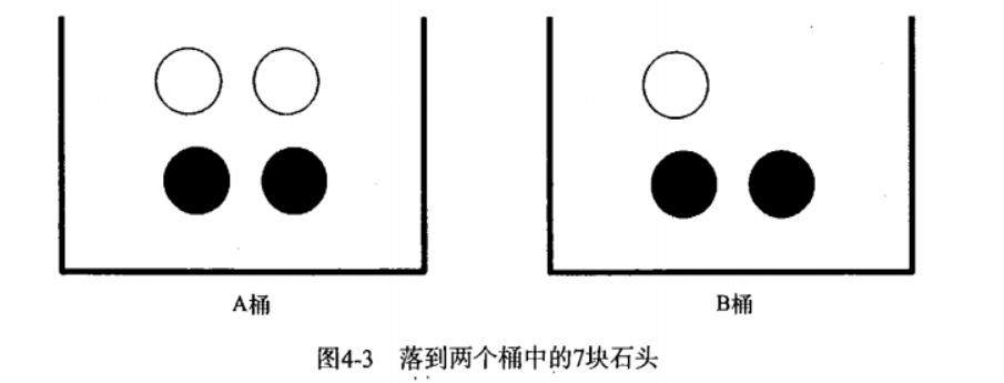
Seven stones are placed in two barrels as shown in the figure. How should the conditional probability be calculated  ？

To calculate P(white) or P(black), obviously, the information of the bucket where the stone is located will change the result, which is the conditional probability. Assuming that the calculation is the probability of taking the white stone from bucket B, this probability can be recorded as P (white|bucket b), which we call "the probability of taking the white stone when the stone is known to come from bucket B".

It is easy to get that the value of P (white|bucket a) is 2 / 4 and the value of P (white|bucket b) is 1 / 3.

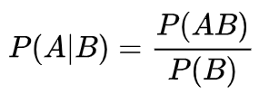
The calculation formula of conditional probability is as follows:

 

Put it in our example: P (white|bucket b) = P (white and bucket B) / P (bucket B)

Formula interpretation:

P (white|bucket b): the probability of taking out white stone under the condition that the stone is known to come from bucket B
P (white and bucket B): probability of taking out the white stone in bucket B = 1 / 7
P (bucket B): the probability of taking out the stone in bucket B is 3 / 7
 

3. Bayesian theorem

Another effective method to calculate conditional probability is called Bayesian theorem. Bayesian theorem tells us how to exchange the conditions and results in conditional probability, that is, if known   P(X|Y), requirements   P(Y|X):

P(Y∣X)=P(X∣Y)P(Y)​/P(X)

P(Y): a priori probability. A priori probability means that something has not happened yet. It is a priori probability to find the possibility of this thing happening. It often appears as "cause" in the problem of "seeking result from cause".

P (Y ∣ X) P (Y | X) P (Y ∣ X): a posteriori probability. A posteriori probability refers to the probability that something has happened and the reason for it is caused by a certain factor. The calculation of a posteriori probability should be based on a priori probability

P (x ∣ Y) P (x | Y) P (x ∣ Y): conditional probability, also known as likelihood probability, is generally obtained through historical data statistics. Generally, it is not called a priori probability, but it also conforms to the a priori definition.

4. Naive Bayesian classifier

The naive Bayesian method learns the joint probability distribution P (x, y) P (x, y) P (x, y) through the training data set, which is actually learning the prior probability distribution and conditional probability distribution:

A priori probability distribution:

Conditional probability distribution:

  Therefore, the joint probability distribution can be obtained from the conditional probability formula  

In naive Bayesian classification, for a given input x, the posterior probability distribution P(Y = c_k|X = x) is calculated through the above learned model, and the class with the largest posterior probability is taken as the output of the class of X. The posterior probability is calculated according to Bayesian theorem:

Apply the full probability formula to the denominator:

 

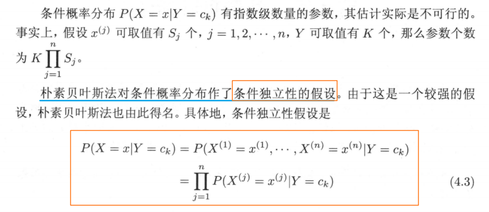
Bring conditional independence hypothesis 4.3 into the above formula to obtain the basic formula of naive Bayesian classification:

 

The denominator in the above formula is the same for all categories and will not affect the calculation results. Therefore, the naive Bayesian classifier can be simplified to

 

3, Spam filtering

1. Steps of realizing spam classification by naive Bayes

(1) Collect data: provide text files.

(2) Prepare data: parse the text file into an entry vector.

(3) Analyze data: check entries to ensure the correctness of parsing.

(4) Training algorithm: calculate the conditional probability of different independent features.

(5) Test algorithm: calculate the error rate.

(6) Using algorithms: build a complete program to classify a group of documents

2. Data set download

There are two folders ham and spam under the email folder: Click to download the dataset

txt file in ham folder is normal mail;

txt file under spam file is spam;

3. Code implementation

# -*- coding: UTF-8 -*-
import numpy as np
import re
import random
 
 
 
"""
Function description:The segmented experimental sample entries are sorted into a list of non repeated entries, that is, a vocabulary
Parameters:
    dataSet - Collated sample data set
Returns:
    vocabSet - Returns a list of non repeating entries, that is, a glossary
"""
def createVocabList(dataSet):
    vocabSet = set([])  # Create an empty non repeating list
    for document in dataSet:
        vocabSet = vocabSet | set(document)  # Union set
    return list(vocabSet)
 
 
"""
Function description:according to vocabList Glossary, adding inputSet Vectorization, each element of the vector is 1 or 0
Parameters:
    vocabList - createVocabList List of returned
    inputSet - Segmented entry list
Returns:
    returnVec - Document vector,Word set model
"""
def setOfWords2Vec(vocabList, inputSet):
    returnVec = [0] * len(vocabList)               #Create a vector with 0 elements
    for word in inputSet:                          #Traverse each entry
        if word in vocabList:                      #If the entry exists in the vocabulary, set 1
            returnVec[vocabList.index(word)] = 1
        else:
            print("the word: %s is not in my Vocabulary!" % word)
    return returnVec        #Return document vector
 
 
"""
Function description:according to vocabList Vocabulary, constructing word bag model
Parameters:
    vocabList - createVocabList List of returned
    inputSet - Segmented entry list
Returns:
    returnVec - Document vector,Word bag model
"""
def bagOfWords2VecMN(vocabList, inputSet):
    returnVec = [0] * len(vocabList)  # Create a vector with 0 elements
    for word in inputSet:             # Traverse each entry
        if word in vocabList:         # If the entry exists in the vocabulary, the count is incremented by one
            returnVec[vocabList.index(word)] += 1
    return returnVec  # Return word bag model
 
 
"""
Function description:Naive Bayesian classifier training function
Parameters:
    trainMatrix - Training document matrix, i.e setOfWords2Vec Returned returnVec Composition matrix
    trainCategory - Training category label vector, i.e loadDataSet Returned classVec
Returns:
    p0Vect - Conditional probability array of normal mail class
    p1Vect - Conditional probability array of spam class
    pAbusive - Probability that the document belongs to spam
"""
def trainNB0(trainMatrix, trainCategory):
    numTrainDocs = len(trainMatrix)  # Calculate the number of training documents
    numWords = len(trainMatrix[0])  # Calculate the number of entries per document
    pAbusive = sum(trainCategory) / float(numTrainDocs)  # Probability that the document belongs to spam
    p0Num = np.ones(numWords)
    p1Num = np.ones(numWords)  # Create numpy.ones array, initialize the number of entries to 1, and Laplace smoothing
    p0Denom = 2.0
    p1Denom = 2.0  # Denominator initialized to 2, Laplace smoothing
    for i in range(numTrainDocs):
        if trainCategory[i] == 1:  # The data required for statistics of conditional probability belonging to insult class, i.e. P(w0|1),P(w1|1),P(w2|1)···
            p1Num += trainMatrix[i]
            p1Denom += sum(trainMatrix[i])
        else:  # The data required to count the conditional probability belonging to the non insult class, i.e. P(w0|0),P(w1|0),P(w2|0)···
            p0Num += trainMatrix[i]
            p0Denom += sum(trainMatrix[i])
    p1Vect = np.log(p1Num / p1Denom)
    p0Vect = np.log(p0Num / p0Denom)   #Take logarithm to prevent lower overflow
    return p0Vect, p1Vect, pAbusive  # Return the conditional probability array belonging to normal mail class, the conditional probability array belonging to insulting spam class, and the probability that the document belongs to spam class
 
 
"""
Function description:Naive Bayesian classifier classification function
Parameters:
	vec2Classify - Array of entries to be classified
	p0Vec - Conditional probability array of normal mail class
	p1Vec - Conditional probability array of spam class
	pClass1 - Probability that a document is spam
Returns:
	0 - It belongs to normal mail class
	1 - Belong to spam
"""
def classifyNB(vec2Classify, p0Vec, p1Vec, pClass1):
    #p1 = reduce(lambda x, y: x * y, vec2Classify * p1Vec) * pClass1  # Multiply corresponding elements
    #p0 = reduce(lambda x, y: x * y, vec2Classify * p0Vec) * (1.0 - pClass1)
    p1=sum(vec2Classify*p1Vec)+np.log(pClass1)
    p0=sum(vec2Classify*p0Vec)+np.log(1.0-pClass1)
    if p1 > p0:
        return 1
    else:
        return 0
 
"""
Function description:Receives a large string and parses it into a list of strings
"""
def textParse(bigString):  # Convert string to character list
    listOfTokens = re.split(r'\W*', bigString)  # Use special symbols as segmentation marks to segment strings, that is, non alphabetic and non numeric
    return [tok.lower() for tok in listOfTokens if len(tok) > 2]  # Except for a single letter, such as a capital I, other words become lowercase
 
 
"""
Function description:Test naive Bayes classifier and use naive Bayes for cross validation
"""
def spamTest():
    docList = []
    classList = []
    fullText = []
    for i in range(1, 26):  # Traverse 25 txt files
        wordList = textParse(open('email/spam/%d.txt' % i, 'r').read())  # Read each spam and convert the string into a string list
        docList.append(wordList)
        fullText.append(wordList)
        classList.append(1)  # Mark spam, 1 indicates junk file
        wordList = textParse(open('email/ham/%d.txt' % i, 'r').read())  # Read each non spam message and convert the string into a string list
        docList.append(wordList)
        fullText.append(wordList)
        classList.append(0)  # Mark normal mail, 0 indicates normal file
    vocabList = createVocabList(docList)  # Create vocabulary without repetition
    trainingSet = list(range(50))
    testSet = []  # Create a list that stores the index values of the training set and the test set
    for i in range(10):  # From the 50 emails, 40 were randomly selected as the training set and 10 as the test set
        randIndex = int(random.uniform(0, len(trainingSet)))  # Random selection of index value
        testSet.append(trainingSet[randIndex])  # Add index value of test set
        del (trainingSet[randIndex])  # Delete the index value added to the test set in the training set list
    trainMat = []
    trainClasses = []  # Create training set matrix and training set category label coefficient vector
    for docIndex in trainingSet:  # Ergodic training set
        trainMat.append(setOfWords2Vec(vocabList, docList[docIndex]))  # Add the generated word set model to the training matrix
        trainClasses.append(classList[docIndex])  # Add a category to the training set category label coefficient vector
    p0V, p1V, pSpam = trainNB0(np.array(trainMat), np.array(trainClasses))  # Training naive Bayesian model
    errorCount = 0  # Error classification count
    for docIndex in testSet:  # Traversal test set
        wordVector = setOfWords2Vec(vocabList, docList[docIndex])  # Word set model of test set
        if classifyNB(np.array(wordVector), p0V, p1V, pSpam) != classList[docIndex]:  # If the classification is wrong
            errorCount += 1  # Error count plus 1
            print("Misclassified test sets:", docList[docIndex])
    print('Error rate:%.2f%%' % (float(errorCount) / len(testSet) * 100))
 
 
if __name__ == '__main__':
    spamTest()

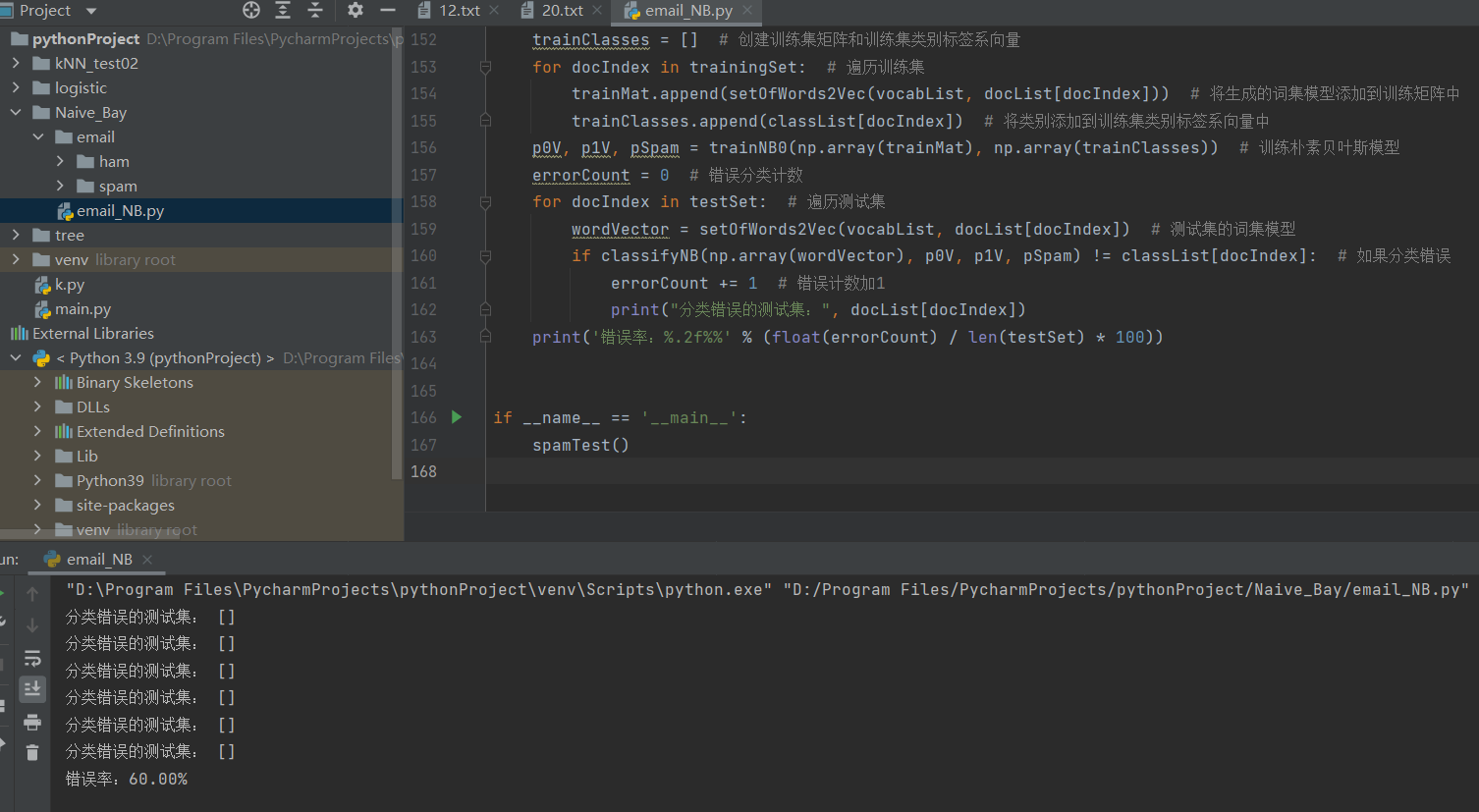
  4. Operation results

 

5. Naive Bayesian evaluation

Advantages: it is still effective in the case of less data, and can deal with multi category problems

Disadvantages: it is sensitive to the preparation method of input data; Because of simplicity Bayes Because of its "simplicity" characteristics, it will bring some loss of accuracy