Since the development of computer algorithms, there have been many different classifications. At present, the most widely used is the generalized swarm intelligent optimization algorithm. For example, particle swarm optimization (PSO), whale optimization (WOA), gray wolf optimization (GWO), dragonfly optimization (DA), universe optimization (MVO), moth fire optimization (MFO), grasshopper optimization, etc.

      We can browse the specific explanations of these algorithms on different learning websites, such as CSDN, Zhihu, etc. I will not repeat the explanation of specific algorithms here. I want to describe the common laws of these algorithms here, so as to help students have a better understanding of this part.

    Common points of swarm intelligence optimization algorithms:

  1. Random initialization

function X=initialization(SearchAgents_no,dim,ub,lb)%SearchAgents_no Is the population number; dim Dimension of problem solving; ub Upper bound of variable; lb Lower bound of variable

Boundary_no= size(ub,2); % numnber of boundaries

% If the boundaries of all variables are equal and user enter a signle
% number for both ub and lb
if Boundary_no==1
    X=rand(SearchAgents_no,dim).*(ub-lb)+lb;
end

% If each variable has a different lb and ub
if Boundary_no>1
    for i=1:dim
        ub_i=ub(i);
        lb_i=lb(i);
        X(:,i)=rand(SearchAgents_no,1).*(ub_i-lb_i)+lb_i;
    end
end

For a problem we want to solve, we must first understand the dimensions of solving the problem, which can be roughly understood as several X. for example, if we have two X (X1, x2), the dimension of the problem we want to solve is 2. In the source code, we need to specify the range of variable x. different x can have different ranges. Of course, according to the actual problem, all variables The range of (X1, X2,..., Xn) can also be consistent. In the above code, lb and ub are presented. In the above code, the number of groups is specified as SearchAgents_no. generally, the number of populations in the original algorithm is 30, so the result of the random initialization process can be understood as a matrix of 30 rows and N columns (the dimension of solving the problem is n).

In the setting process, there is another important parameter - Max_iteration. There are two termination conditions for the algorithm, one is convergence accuracy (if the convergence decline does not exceed the set threshold within a certain period of time, it is almost optimal and there is no need to continue.) The other is the maximum number of iterations, which is used as the final iteration termination condition in general algorithms. The specific values can be set by reference according to the corresponding references.

For a specific problem, the dimension of the problem (dim), the upper and lower boundaries of variables, and the population number can be set according to the actual situation. When the original code is proposed, there will be a series of test functions to verify

[lb,ub,dim,fobj]=Get_Functions_details(Function_name);

The above code is to extract the dimension, variable upper and lower boundaries, and objective function from the test function. The objective function is described in detail in the following content.

2. Specific process of algorithm

Before the algorithm enters the iterative cycle, that is, before the continuous optimization process, the fitness of the previous randomized initial matrix will be calculated. If the population number is 30, there are 30 fitness values. By comparing their sizes, take the minimum (or maximum, generally minimum) as the initial optimal fitness value and enter the subsequent iterative optimization for calculation.

for i=1:size(Positions,1)
    Fitness(1,i)=fobj(Positions(i,:));
end

The above code shows that the fitness values of all populations are calculated before iterative optimization.

It is worth mentioning that the concept of fitness value can be simply understood as the value of each population (each row vector) calculated through the objective function formula.

two point one   Global exploration and local development

The two stages of global exploration and local development determine the search quality of the algorithm. They are interconnected. First, conduct global and large-scale search, and then execute small-scale (local) after a certain stage As for how to carry out global search and local development, the logic of each algorithm is different, which can be analyzed in combination with the code. There is a transition between global exploration and local development, that is, when the algorithm is executed, from global exploration to local development. This transition stage exists in almost every algorithm logic. Here, HHO (Harris Eagle) The algorithm and SSA algorithm are introduced as examples.

In HHO algorithm, the energy of prey is used to complete this transition process. Its model is as follows:

                                                  

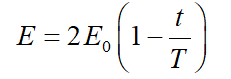
In the above formula, e represents the escape energy of prey,   E0 represents the initial state of energy intensity. T is the maximum number of iterations, and t is the actual number of iterations of the algorithm, which is used as the stop criterion of conventional HHO.

In SSA algorithm,

                                                      

In the above formula, T represents the current iteration and T represents the maximum number of iterations. Parameters play an important role in establishing an appropriate balance between exploration and development trends.

The above is the concrete manifestation of the transition of the two algorithms from global exploration to local development. Different algorithms have different transition forms according to different logic.

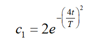
As for the specific implementation of global exploration and local development, various algorithms are the Eight Immortals crossing the sea. At present, most generalized swarm intelligence algorithms are summarized based on biological foraging or survival / life rules. You can refer to the original papers of various algorithms for detailed interpretation. Here is a simple example of the bottle sea squirt algorithm.

while l<Max_iter+1/Maximum iteration limit set
    
    c1 = 2*exp(-(4*l/Max_iter)^2); % Eq. (3.2) in the paper/Global exploration and local development transition
    
    for i=1:size(SalpPositions,1)
        
        SalpPositions= SalpPositions';
        
        if i<=N/2   /Here, according to the foraging characteristics of bottlenose sea squirt, the population is divided into two categories: leader and follower. Firstly, the leader's position is updated.
            for j=1:1:dim
                c2=rand();
                c3=rand();
                %%%%%%%%%%%%% % Eq. (3.1) in the paper %%%%%%%%%%%%%%
                if c3<0.5 
                    SalpPositions(j,i)=FoodPosition(j)+c1*((ub(j)-lb(j))*c2+lb(j));
                else
                    SalpPositions(j,i)=FoodPosition(j)-c1*((ub(j)-lb(j))*c2+lb(j));
                end
                %%%%%%%%%%%%%%%%%%%%%%%%%%%%%%%%%%%%%%%%%%%%%%%%%%%%%%
            end
            
        elseif i>N/2 && i<N+1   /Update the location of followers again.
            point1=SalpPositions(:,i-1);
            point2=SalpPositions(:,i);
            
            SalpPositions(:,i)=(point2+point1)/2; % % Eq. (3.4) in the paper
        end
        
        SalpPositions= SalpPositions';
    end
    
    for i=1:size(SalpPositions,1)  /After the update, the boundary conditions shall be defined.
        
        Tp=SalpPositions(i,:)>ub';Tm=SalpPositions(i,:)<lb';SalpPositions(i,:)=(SalpPositions(i,:).*(~(Tp+Tm)))+ub'.*Tp+lb'.*Tm;
        
        SalpFitness(1,i)=fobj(SalpPositions(i,:));
        
        if SalpFitness(1,i)<FoodFitness
            FoodPosition=SalpPositions(i,:);
            FoodFitness=SalpFitness(1,i);
            
        end
    end
    
    Convergence_curve(l)=FoodFitness;/The fitness value of the obtained individual is stored and placed in the convergence curve
    l = l + 1;/Mark the number of iterations, and the iterations are accumulated.
end

When executing the while loop, the individual fitness values are continuously compared. After the iteration is completed, the best fitness value is obtained.

Here, the whole process of the algorithm is generally clear, and the main parameters and processes are described above.

The problem of objective function has been mentioned above. For different practical problems, the setting of natural objective function is different, so it is necessary to write relevant programs. In order to facilitate the test of algorithm performance, relevant scholars have written standard test functions.

function [lb,ub,dim,fobj] = Get_Functions_details(F)


switch F
    case 'F1'
        fobj = @F1;
        lb=-100;
        ub=100;
        dim=30;
        
    case 'F2'
        fobj = @F2;
        lb=-10;
        ub=10;
        dim=10;
        
    case 'F3'
        fobj = @F3;
        lb=-100;
        ub=100;
        dim=10;

end

end

% F1

function o = F1(x)
o=sum(x.^2);
end

% F2

function o = F2(x)
o=sum(abs(x))+prod(abs(x));
end

% F3

function o = F3(x)
dim=size(x,2);
o=0;
for i=1:dim
    o=o+sum(x(1:i))^2;
end
end

The above shows three standard test functions from F1 to F3. You can see that in Get_Functions_details, we read the boundary, dimension and objective function of the function. The objective function here uses the skill of @ and the specific function form is also given in the form of function o = F(x).

The general algorithm flow is basically the same. If you need some algorithm programs or don't understand them, you can discuss them in private letters and learn together.