Sample imbalance in binary SVC: an important parameter class_weight
For the classification problem, one of the pain points that can never escape is the sample imbalance problem. Sample imbalance refers to a class of labels in a set of data sets It accounts for a large proportion, but we have the situation to capture the needs of a specific classification. For example, we now need to classify potential criminals and ordinary people. The proportion of potential criminals in the total population is quite low, perhaps only about 2%, 98% of people are ordinary people, and our goal is to capture potential criminals. Such label distribution will bring many problems.
First, the classification model naturally tends to most classes, making it easier for most classes to be judged correctly and a few classes to be sacrificed. Because for the model, the larger the sample size, the more information the label can learn, and the algorithm will rely more on the information learned from most classes for judgment. If we want to capture a few classes, the model will fail. Secondly, the model evaluation index will lose its meaning. In this classification situation, even if the model does nothing and treats everyone as a person who will not commit a crime, the accuracy can be very high, which makes the model evaluation index accuracy meaningless and can not achieve our modeling goal of "identifying people who will commit a crime".
So now, we should first make the algorithm realize that the labels of data are unbalanced, and make the model model model in the direction of capturing a few classes by imposing some penalties or changing the sample itself. Then, we need to improve our model evaluation indicators and use more targeted indicators for a few classes to optimize the model.
To solve the first problem, we have introduced some basic methods in logistic regression, such as up sampling and down sampling. However, these sampling methods will increase the total number of samples. For the algorithm of support vector machine, which always has a great impact on the calculation speed, we don't want to easily increase the number of samples. Moreover, the decision-making in support vector machine is only affected by the decision boundary, and the decision boundary is only affected by parameter C and support vector. Simply increasing the number of samples will not only increase the calculation time, but also increase countless sample points that have no impact on the decision boundary. Therefore, in support vector machine, we should rely heavily on the parameter we adjust the sample equilibrium: class in SVC class_weight and sample that can be set in the interface "t"_ weight.
In logistic regression, the parameter class_weight defaults to None. This mode means that it is assumed that all labels in the dataset are balanced, that is, the proportion of labels is automatically considered to be 1:1. Therefore, when the samples are unbalanced, we can use a dictionary such as {"tag value 1": weight 1, "tag value 2": weight 2} to input the real sample tag proportion to make the algorithm realize that the samples are unbalanced. Or use the "balanced" mode and directly use n_samples/(n_classes) * np.bincount(y)) as the weight can better correct our sample imbalance.
However, in SVM, our classification judgment is based on the decision boundary, and the parameter that ultimately determines what support vector to use and the decision boundary is parameter C, so all sample equilibria are adjusted through parameter C.
SVC parameter: class_weight
You can enter a dictionary or "balanced", or leave it blank. The default is None to SVC, and the parameter C of class I is set to class_weight [i] * C. If no specific class_weight is given, all classes are assumed to have the same weight 1, and the model will be trained according to the original condition of the data. If you want to improve the sample imbalance, please enter a dictionary such as {tag value 1 ": weight 1," tag value 2 ": weight 2}, and the parameter C will be automatically set to C: weight 1 of tag value 1 * C. Value of label: weight 2*C.
Alternatively, you can use the "balanced" mode, which uses the value of y to automatically adjust the weight inversely proportional to the class frequency in the input data to n_samples/(n_classes) * np.bincount(y))
Parameter of SVC interface "t": sample_weight
Array with structure (n_samples, ), It must correspond to each sample of the characteristic matrix in the input "t"
The weight of each sample at "t", let the weight * The C value corresponding to each sample forces the classifier to emphasize the samples with larger weight. Usually, the larger weight is added to the samples of a few classes to force the model to model in the direction of a few classes
Generally speaking, we only select one of these two parameters to set. If we set two parameters at the same time, C will be affected by both parameters at the same time, Namely Weight set in class_weight * Weight set in sample_weight * C.
Let's take a look at how to use this parameter.
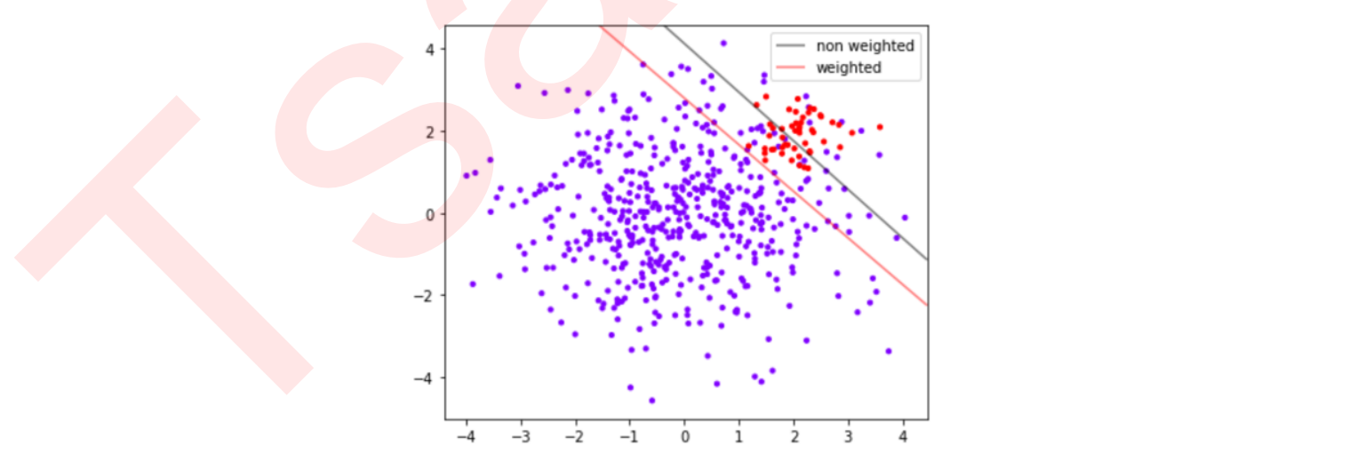
First, we build a set of data sets with unbalanced samples. We build two SVC models on this set, one with class_weight parameter and the other without class_weight parameter. We evaluate the two models and draw their decision boundaries to observe the effect of class_weight.
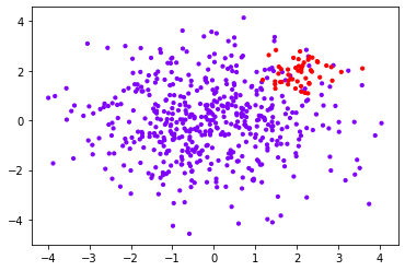
import numpy as np
import matplotlib.pyplot as plt
from sklearn import svm
from sklearn.datasets import make_blobs

class_1 = 500 #Category 1 has 500 samples
class_2 = 50 #Category 2 has only 50
centers = [[0.0, 0.0], [2.0, 2.0]] #Set the center of two categories
clusters_std = [1.5, 0.5] #Set the variance of the two categories. Generally speaking, the category with large sample size will be more loose
X, y = make_blobs(n_samples=[class_1, class_2], centers=centers, cluster_std=clusters_std, random_state=0, shuffle=False)

#See what the dataset looks like
plt.scatter(X[:, 0], X[:, 1], c=y, cmap="rainbow",s=10)
#Among them, red dots are a few categories and purple dots are most categories
#Do not set class_weight
clf = svm.SVC(kernel='linear', C=1.0)
clf.fit(X, y)

#Set class_weight
wclf = svm.SVC(kernel='linear', class_weight={1: 10})
wclf.fit(X, y)

#Score the two models separately. This score is the accuracy
print(clf.score(X,y))
wclf.score(X,y)
result:
0.9418181818181818
0.9127272727272727
Draw the decision boundary of data under the two models
#First, there must be data distribution
plt.figure(figsize=(6,5))
plt.scatter(X[:,0], X[:,1], c=y, cmap="rainbow",s=10)
ax = plt.gca()
#Get the current subgraph. If it does not exist, create a new subgraph
#The first step in drawing decision boundaries: have a grid

xlim = ax.get_xlim()
ylim = ax.get_ylim()

xx = np.linspace(xlim[0], xlim[1], 30)
yy = np.linspace(ylim[0], ylim[1], 30)
YY, XX = np.meshgrid(yy, xx)
xy = np.vstack([XX.ravel(), YY.ravel()]).T

#Step 2: find out the distance from our sample point to the decision boundary
Z_clf = clf.decision_function(xy).reshape(XX.shape)
a = ax.contour(XX, YY, Z_clf, colors='black', levels=[0], alpha=0.5, linestyles=['-'])

Z_wclf = wclf.decision_function(xy).reshape(XX.shape)
b = ax.contour(XX, YY, Z_wclf, colors='red', levels=[0], alpha=0.5, linestyles=['-'])

#Step 3: draw legend
plt.legend([a.collections[0], b.collections[0]], ["non weighted" , "weighted"],loc="upper right")
plt.show()
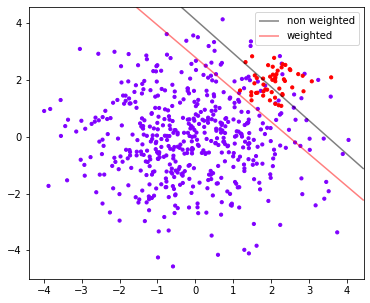 It can be seen that from the perspective of accuracy, the accuracy is higher without sample balance, and the accuracy becomes lower after sample balance. This is because After sample balancing, in order to capture a few classes more effectively, the model wrongly hurts many samples of most classes, and the number of samples of most classes is wrongly divided > Now, if our goal is to improve the overall accuracy of the model, we must reject the sample balance and use the model before class_weight is set.
However, in reality, we often pursue to capture minority classes, because in many cases, the cost of misjudging minority classes is huge. For example, we mentioned the example of judging potential criminals and ordinary people. If we can't identify potential criminals, these people may harm the society and cause adverse effects. However, if we mistake ordinary people for potential criminals, we may just need to increase the cost of monitoring and artificial screening. So for us, we would rather misjudge ordinary people than let go of any potential offender. If we want to capture a few classes at all costs, or if we want to capture as many minority classes as possible, we must use class_ Model after weight setting.
Model evaluation index of SVC
As can be seen from the example in the previous section, if our goal is to capture as few classes as possible, the model evaluation of accuracy will gradually fail, so we need new model evaluation indicators to help us. In fact, we only need to check the accuracy of the model on a few classes. As long as we can capture a few classes as much as possible, we can achieve our goal.
However, at this time, new problems arise again. After we make a wrong judgment on most classes, we will need manual screening or more business measures to eliminate the most classes we make a wrong judgment one by one. This behavior is often accompanied by a high cost. For example, when a bank judges "whether a customer applying for a credit card will default", if a customer is judged as "will default", the customer's credit card application will be rejected. In order to catch the "will default" people, a large number of "will not default" customers are judged as "will default" "Many innocent customers' applications will be rejected. Credit cards mean interest income to banks, and it will be a huge loss to banks to refuse many customers who would not have defaulted. Similarly, when Volkswagen recalls cars that do not meet the EU standards, in order to find all cars that do not meet the standards, it will put a pile of cars that would have met the standards The cost of car recall is immeasurable.
In other words, if we simply pursue to capture a few classes, the cost will be too high without considering the few classes, and we will not be able to achieve the effect of the model. Therefore, in reality, we often look for a balance between the ability to capture a few classes and the cost to pay after judging most classes wrong. If a model can capture as few classes as possible In order to evaluate this ability, we will introduce a new model evaluation index: confusion matrix and ROC curve to help us.
Confusion matrix Matrix)
Confusion matrix is a multi-dimensional measurement index system for binary classification problems, which is extremely useful in case of sample imbalance. In confusion matrix, we regard a few classes as positive examples and most classes as negative examples. In ordinary classification algorithms such as decision tree and random forest, that is, the minority class is 1 and the majority class is 0. In SVM, that is, the minority class is 1 and the majority class is - 1. Ordinary confusion matrix Confusion matrix is generally represented by {0,1}. Confusion matrix, as its name, is very confusing. In many textbooks, various names and definitions in confusion matrix are difficult to understand and remember. I have found a simplified way to display the confusion matrix of standard two categories, as shown in the figure:
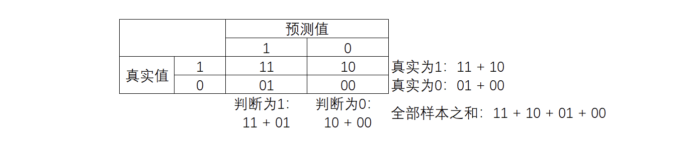
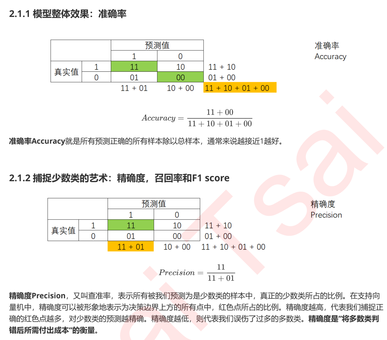
In the confusion matrix, the real value always comes first and the predicted value comes last. In fact, it can be easily seen that the diagonals of 11 and 00 are all correctly predicted, and the diagonals of 01 and 10 are all wrong predicted. Based on the confusion matrix, we have six different model evaluation indicators, and the range of these evaluation indicators is [0,1] Between, all indicators with 11 and 00 as molecules are closer to 1, so the indicators with 01 and 10 as molecules are closer to 0, the better. For all indicators, we use orange to represent the denominator and green to represent the molecule, then we have:
Accuracy
#For the grey decision boundary without class_weight and sample balance:
print((y[y == clf.predict(X)] == 1).sum()/(clf.predict(X) == 1).sum())
#For the red decision boundary with class_weight and sample balance:
(y[y == wclf.predict(X)] == 1).sum()/(wclf.predict(X) == 1).sum()
result:
0.7142857142857143
0.5102040816326531
Accuracy is also called precision, that is, the proportion of red points in all points above the decision boundary
It can be seen that after sample balancing, the accuracy decreases. Because it is obvious that after sample balancing, more purple spots of most classes are injured by us. Accuracy can help us judge whether the prediction of a few classes is accurate every time, so it is also called "precision". In reality, the sample is unbalanced
recall
#Proportion of all points with predict 1 / all points with predict 1
#For the grey decision boundary without class_weight and sample balance:
print((y[y == clf.predict(X)] == 1).sum()/(y == 1).sum())

#For the red decision boundary with class_weight and sample balance:
(y[y == wclf.predict(X)] == 1).sum()/(y == 1).sum()
0.6
1.0
If we want to find a few categories at all costs (such as the example of potential offenders), we will pursue a high recall rate. On the contrary, if our goal is not to capture a few categories as much as possible, we don't need to care about the recall rate.
Note that the numerator of recall rate and accuracy is the same (both are 11), but the denominator is different. Recall rate and accuracy fluctuate, and there is no difference between the two Balance represents the balance between capturing the needs of the minority and trying not to hurt the needs of the majority. Which side we prefer depends on our business needs: whether it is more expensive to hurt the majority or not to capture the minority.
F1 score
In order to take into account both accuracy and recall, we created the harmonic average of the two as a comprehensive index to consider the balance between the two, which is called F1 measure. The harmonic average between the two numbers tends to be close to the smaller of the two numbers, so we pursue F1 as high as possible measure, It can ensure that our accuracy and recall rate are relatively high. F1 Measure is distributed between [0,1]. The closer it is to 1, the better.
 False Negative Rate, which is equal to 1 - Recall.
Specificity and false positive rate
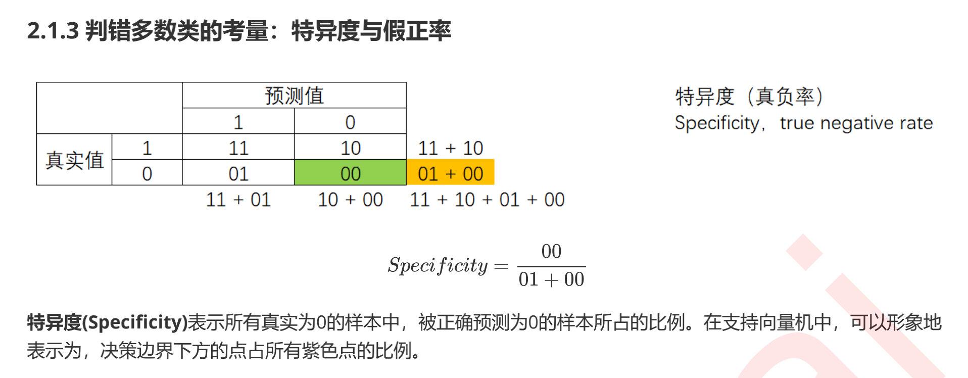
#All samples correctly predicted as 0 / all 0 samples
#No class for_ Weight, for the grey decision boundary without sample balance:
print((y[y == clf.predict(X)] == 0).sum()/(y == 0).sum())

#For classes with_ Weight, the red decision boundary of sample balance:
(y[y == wclf.predict(X)] == 0).sum()/(y == 0).sum()
result:
0.976
0.904
Confusion matrix
sklearn provides a large number of classes to help us understand and use confusion matrices.
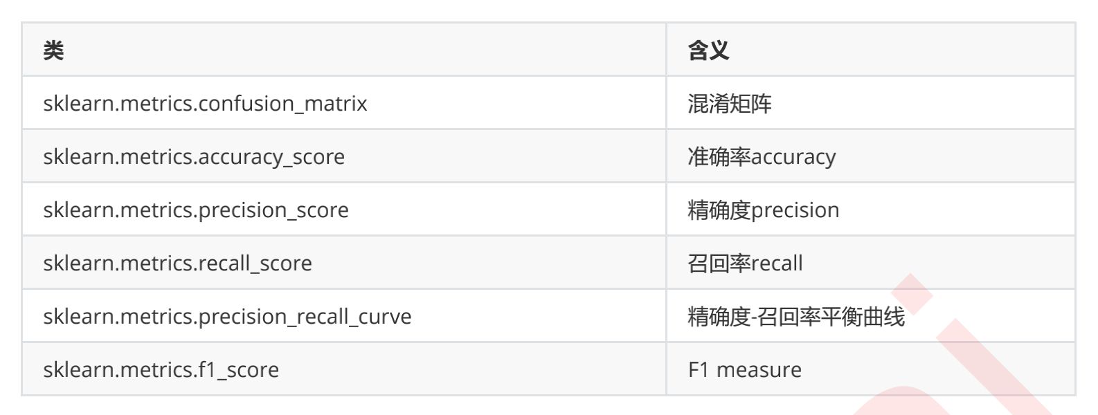
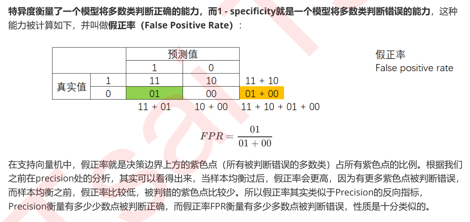
Based on the confusion matrix, we learned a total of six indicators: Accuracy, Precision, Recall, and the balance index F of Accuracy and Recall measure, specificity fi city, and false positive rate FPR. Among them, the false positive rate has a very important application: when we pursue higher Recall, Precision will decline, that is, as more minority classes are captured, more majority classes will be judged incorrectly. However, we are curious about how the model's ability to judge most classes incorrectly will change with the gradual increase of Recall?
We want to understand that for every minority class I judge correctly, how many majority classes will be judged incorrectly. The false positive rate can help us measure the change of this ability. In contrast, Precision cannot determine the proportion of most classes with wrong judgment in all most classes, so it cannot take into account the overall Accuracy of the model in the process of promoting Recall. Therefore, we can use the balance between Recall and FPR to replace the balance between Recall and Precision. Let's measure how the model mistakenly damages most classes when trying to capture a few classes. This is the balance measured by our ROC curve.
ROC curve, The Receiver Operating Characteristic Curve, translated as subject operating Characteristic Curve. This is a curve with The false positive rate FPR under different thresholds as The abscissa and The Recall rate Recall under different thresholds as The ordinate. Let's start with probability and threshold.
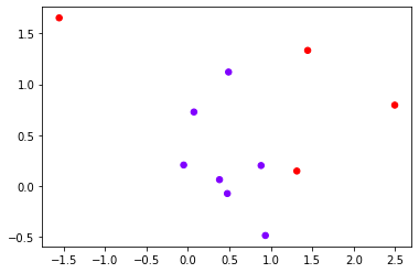
class_1_ = 7
class_2_ = 4
centers_ = [[0.0, 0.0], [1,1]]
clusters_std = [0.5, 1]
X_, y_ = make_blobs(n_samples=[class_1_, class_2_],
centers=centers_,
cluster_std=clusters_std ,
random_state=0, shuffle=False)
plt.scatter(X_[:, 0], X_[:, 1], c=y_, cmap="rainbow",s=30)
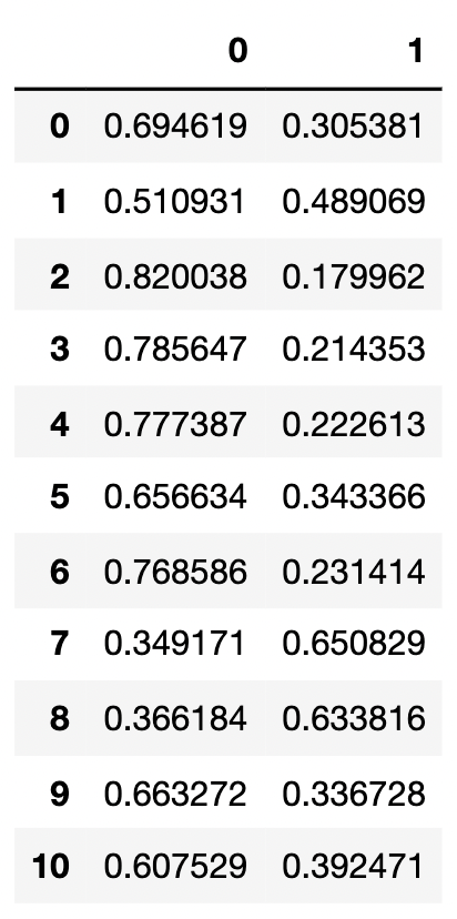
from sklearn.linear_model import LogisticRegression as LogiR
clf_lo = LogiR().fit(X_,y_)

prob = clf_lo.predict_proba(X_)

#Put the sample and probability into a DataFrame
import pandas as pd
prob = pd.DataFrame(prob)
prob.columns = ["0","1"]

prob
#Manually adjust the threshold to change the effect of our model
for i in range(prob.shape[0]):
    if prob.loc[i,"1"] > 0.5:
        prob.loc[i,"pred"] = 1
    else:
        prob.loc[i,"pred"] = 0
prob["y_true"] = y_
prob = prob.sort_values(by="1",ascending=False)
prob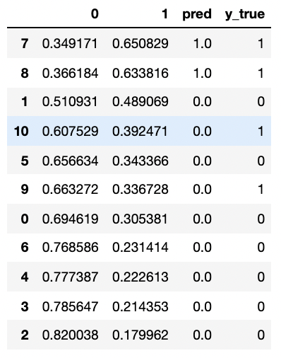
from sklearn.metrics import confusion_matrix as CM, precision_score as P, recall_score as R

print(CM(prob.loc[:,"y_true"],prob.loc[:,"pred"],labels=[1,0])) #1 is a minority class (before writing) 0 is a majority class
#Try manually calculating Precision and Recall?
print(P(prob.loc[:,"y_true"],prob.loc[:,"pred"],labels=[1,0]))
R(prob.loc[:,"y_true"],prob.loc[:,"pred"],labels=[1,0])
[[2 2]
 [0 7]]
1.0
0.5
for i in range(prob.shape[0]):
    if prob.loc[i,"1"] > 0.4:
        prob.loc[i,"pred"] = 1
    else:
        prob.loc[i,"pred"] = 0

print(CM(prob.loc[:,"y_true"],prob.loc[:,"pred"],labels=[1,0]))
print(P(prob.loc[:,"y_true"],prob.loc[:,"pred"],labels=[1,0]))
print(R(prob.loc[:,"y_true"],prob.loc[:,"pred"],labels=[1,0]))
[[2 2] [1 6]] 0.6666666666666666 0.5
It can be seen that our model evaluation indicators will change under different thresholds. We are using this to observe how Recall and FPR affect each other. However, it should be noted that it is not necessary to increase or decrease Recall by increasing the threshold. Everything should be judged according to the actual distribution of data. In order to reflect the influence of threshold, we must first get the prediction probability of classifier in a few classes. For the algorithms that generate likelihood naturally such as logistic regression and naive Bayes, which are algorithms that calculate probability, it is naturally very easy to obtain probability, but for some other classification algorithms, such as decision tree, such as SVM, Their classification is not related to probability. Can't we draw ROC curve on them? and be not so.
The decision tree has leaf nodes. A leaf node may contain samples of different classes. Suppose a sample is included in leaf node a, and node a contains 10 If 6 samples are 1 and 4 samples are 0, the probability of occurrence of positive class 1 in this leaf node is 60%, and the probability of occurrence of Class 0 in this leaf node is 40%. For all samples in this leaf node, the probability of 1 and 0 on the node is the probability of 1 and 0 corresponding to this sample. You can verify it yourself. But think about a problem. Because the decision tree can be drawn very deep, when it is deep enough, each leaf node of the decision tree may not contain labels of multiple categories, and there may be only one label in a leaf, that is, the impurity of the leaf node is 0. At this moment, for each sample, their corresponding "probability" is 0 or 1. At this time, we can't adjust the threshold Section our Recall and FPR. The same is true for random forests.
Therefore, if we have probability requirements, we will give priority to logical regression or naive Bayes. But in fact, SVM can also generate probability. Let's see how it does it.
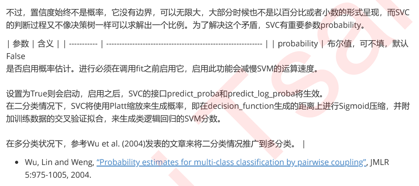
SVM probability prediction: important parameter probability, interface predict_proba and decision_function
We used the SVC interface decision when drawing contours, that is, decision boundaries_ Function, which returns the distance from each sample in the input characteristic matrix to the hyperplane dividing the dataset. In SVM, we use hyperplane to judge our samples. In essence, when the distance between two points is the same symbol, the sample points farther away from the hyperplane have a great probability of belonging to a label class. For example, a point 0.1 away from the hyperplane and a point 100 away from the hyperplane are obviously points with a distance of 0.1, which are more likely to be points of negative category mixed into the boundary. Similarly, for a point with a distance of - 0.1 from the hyperplane and a point with a distance of - 100 from the hyperplane, it is obvious that the label of a point with a distance of - 100 is more likely to be negative. Therefore, the distance to the hyperplane reflects the possibility that the sample belongs to a label class to a certain extent. Interface decision_ The value returned by function is therefore considered as SVM Confidence in (con fi dence).
#Using the initial X and y, the sample is unbalanced in this model
class_1 = 500 #Category 1 has 500 samples
class_2 = 50 #Category 2 has only 50
centers = [[0.0, 0.0], [2.0, 2.0]] #Set the center of two categories
clusters_std = [1.5, 0.5] #Set the variance of the two categories. Generally speaking, the category with large sample size will be more loose
X, y = make_blobs(n_samples=[class_1, class_2],
                centers=centers,
                cluster_std=clusters_std ,
                random_state=0, shuffle=False)

#See what the dataset looks like
plt.scatter(X[:, 0], X[:, 1], c=y, cmap="rainbow",s=10)

#Among them, red dots are a few categories and purple dots are most categories
clf_proba = svm.SVC(kernel="linear",C=1.0,probability=True).fit(X,y)

print(clf_proba.predict_proba(X)) #Generate probabilities under various labels

print(clf_proba.decision_function(X))

print(clf_proba.decision_function(X).shape)
[[0.69850902 0.30149098]
 [0.28868513 0.71131487]
 [0.96116579 0.03883421]
 ...
 [0.17705259 0.82294741]
 [0.38049218 0.61950782]
 [0.34181702 0.65818298]]

[ -0.39182241   0.95617053  -2.24996184  -2.63659269  -3.65243197
  -1.67311996  -2.56396417  -2.80650393  -1.76184723  -4.7948575
  -7.59061196  -3.66174848  -2.2508023   -4.27626526   0.78571364
  -3.24751892  -8.57016271  -4.45823747  -0.14034183  -5.20657114
  -8.02181046  -4.18420871  -5.6222409   -5.12602771  -7.22592707
  -5.07749638  -6.72386021  -3.4945225   -3.51475144  -5.72941551
  -5.79160724  -8.06232013  -4.36303857  -6.25419679  -5.59426696
  -2.60919281  -3.90887478  -4.38754704  -6.46432224  -4.54279979
  -4.78961735  -5.53727469   1.33920817  -2.27766451  -4.39650854
  -2.97649872  -2.26771979  -2.40781748  -1.41638181  -3.26142275
  -2.7712218   -4.87288439  -3.2594128   -5.91189118   1.48676267
   0.5389064   -2.76188843  -3.36126945  -2.64697843  -1.63635284
  -5.04695135  -1.59196902  -5.5195418   -2.10439349  -2.29646147
  -4.63162339  -5.21532213  -4.19325629  -3.37620335  -5.0032094
  -6.04506666  -2.84656859   1.5004014   -4.02677739  -7.07160609
  -1.66193239  -6.60981996  -5.23458676  -3.70189918  -6.74089425
  -2.09584948  -2.28398296  -4.97899921  -8.12174085  -1.52566274
  -1.99176286  -3.54013094  -4.8845886   -6.51002015  -4.8526957
  -6.73649174  -8.50103589  -5.35477446  -5.93972132  -3.09197136
  -5.95218482  -5.87802088  -3.41531761  -1.50581423   1.69513218
  -5.08155767  -1.17971205  -5.3506946   -5.21493342  -3.73358514
  -2.01273566  -3.39045625  -6.34357458  -3.54776648  -0.17804673
  -6.26887557  -4.17973771  -6.68896346  -3.46095619  -5.47965411
  -7.30835247  -4.41569899  -4.95103272  -4.52261342  -2.32912228
  -5.78601433  -4.75347157  -7.10337939  -0.4589064   -7.67789856
  -4.01780827  -4.3031773   -1.83727693  -7.40091653  -5.95271547
  -6.91568411  -5.20341905  -7.19695832  -3.02927263  -4.48056922
  -7.48496425  -0.07011269  -5.80292499  -3.38503533  -4.58498843
  -2.76260661  -3.01843998  -2.67539002  -4.1197355   -0.94129257
  -5.89363772  -1.6069038   -2.6343464   -3.04465464  -4.23219535
  -3.91622593  -5.29389964  -3.59245628  -8.41452726  -3.09845691
  -2.71798914  -7.1383473   -4.61490324  -4.57817871  -4.34638288
  -6.5457838   -4.91701759  -6.57235561  -1.01417607  -3.91893483
  -4.52905816  -4.47582917  -7.84694737  -6.49226452  -2.82193743
  -2.87607739  -7.0839848   -5.2681034   -4.4871544   -2.54658631
  -7.54914279  -2.70628288  -5.99557957  -8.02076603  -4.00226228
  -2.84835501  -1.9410333   -3.86856886  -4.99855904  -6.21947623
  -5.05797444  -2.97214824  -3.26123902  -5.27649982  -3.13897861
  -6.48514315  -9.55083209  -6.46488612  -7.98793665  -0.94456569
  -3.41380968  -7.093158    -5.71901588  -0.88438995  -0.24381463
  -6.78212695  -2.20666714  -6.65580329  -2.56305221  -5.60001636
  -5.43216357  -4.96741585  -0.02572912  -3.21839147   1.13383091
  -1.58640099  -7.57106914  -4.16850181  -6.48179088  -4.67852158
  -6.99661419  -2.1447926   -5.31694653  -2.63007619  -2.55890478
  -6.4896746   -3.94241071  -2.71319258  -4.70525843  -5.61592746
  -4.7150336   -2.85352156  -0.49195707  -8.16191324  -3.80462978
  -6.43680611  -4.58137592  -1.38912206  -6.93900334  -7.7222725
  -8.41592264  -5.613998     0.44396046  -3.07168078  -1.36478732
  -1.20153628  -6.30209808  -6.49846303  -0.60518198  -3.83301464
  -6.40455571  -0.22680504   0.54161373  -5.99626181  -5.98077412
  -3.45857531  -2.50268554  -5.54970836  -9.26535525  -4.22097425
  -0.47257602  -9.33187038  -4.97705346  -1.65256318  -1.0000177
  -5.82202444  -8.34541689  -4.97060946  -0.34446784  -6.95722208
  -7.41413036  -1.8343221   -7.19145712  -4.8082824   -4.59805445
  -5.49449995  -2.25570223  -5.41145249  -5.97739476  -2.94240518
  -3.64911853  -2.82208944  -3.34705766  -8.19712182  -7.57201089
  -0.61670956  -6.3752957   -5.06738146  -2.54344987  -3.28382401
  -5.9927353   -2.87730848  -3.58324503  -7.1488302   -2.63140119
  -8.48092542  -4.91672751  -5.7488116   -3.80044426  -9.27859326
  -2.475992    -6.06980518  -2.90059294  -5.22496057  -5.97575155
  -6.18156775  -5.38363878  -7.41985155  -6.73241325  -4.43878791
  -9.06614408  -1.69153658  -3.71141045  -3.19852116  -4.05473804
  -3.45821856  -4.92039492  -6.55332449  -1.28332784  -4.17989583
  -5.45916562  -3.80974949  -4.27838346  -5.31607024  -0.62628865
  -2.21276478  -3.7397342   -6.66779473  -2.38116892  -2.83460004
  -7.01238422  -2.75282445  -3.01759368  -6.14970454  -6.1300394
  -7.58620719  -3.14051577  -5.82720807  -2.52236034  -7.03761018
  -7.82753368  -8.8447092   -3.11218173  -4.22074847  -0.99624534
  -3.45189404  -1.46956557  -9.42857926  -2.75093993  -0.61665367
  -2.09370852  -9.34768018  -3.39876535  -5.8635608   -2.12987936
  -8.40706474  -3.84209244  -0.5100329   -2.48836494  -1.54663048
  -4.30920238  -5.73107193  -1.89978615  -6.17605033  -3.10487492
  -5.51376743  -4.32751131  -8.20349197  -3.87477609  -1.78392197
  -6.17403966  -6.52743333  -3.02302099  -4.99201913  -5.72548424
  -7.83390422  -1.19722286  -4.59974076  -2.99496132  -6.83038116
  -5.1842235   -0.78127198  -2.88907207  -3.95055581  -6.33003274
  -4.47772201  -2.77425683  -4.44937971  -4.2292366   -1.15145162
  -4.92325347  -5.40648383  -7.37247783  -4.65237446  -7.04281259
  -0.69437244  -4.99227188  -3.02282976  -2.52532913  -6.52636286
  -5.48318846  -3.71028837  -6.91757625  -5.54349414  -6.05345046
  -0.43986605  -4.75951272  -1.82851406  -3.24432919  -7.20785221
  -4.0583863   -3.27842271  -0.68706448  -2.76021537  -5.54119808
  -4.08188794  -6.4244794   -4.76668274  -0.2040958   -2.42898945
  -2.03283232  -4.12879797  -2.70459163  -6.04997273  -2.79280244
  -4.20663028   0.786804    -3.65237777  -3.55179726  -5.3460864
 -10.31959605  -6.69397854  -6.53784926  -7.56321471  -4.98085596
  -1.79893146  -3.89513404  -5.18601688  -3.82352518  -5.20243998
  -3.11707515  -5.80322513  -4.42380099  -5.74159836  -6.6468986
  -3.18053496  -4.28898663  -6.73111304  -3.21485845  -4.79047586
  -4.51550728  -2.70659984  -3.61545839  -7.86496861  -0.1258212
  -7.6559803   -3.15269699  -2.87456418  -6.74876767  -0.42574712
  -7.58877495  -5.30321115  -4.79881591  -4.5673199   -3.6865868
  -4.46822682  -1.45060265  -0.53560561  -4.94874171  -1.26112294
  -1.66779284  -5.57910033  -5.87103484  -3.35570045  -6.25661833
  -1.51564145   0.85085628  -3.82725071  -1.47077448  -3.36154118
  -5.37972404  -2.22844631  -2.78684422  -3.75603932  -1.85645
  -3.33156093  -2.32968944  -5.06053069  -1.73410541  -1.68829408
  -3.79892942  -1.62650712  -1.00001873  -6.07170511  -4.89697898
  -3.66269926  -3.13731451  -5.08348781  -3.71891247  -2.09779606
  -3.04082162  -5.12536015  -2.96071945  -4.28796395  -6.6231135
   1.00003406   0.03907036   0.46718521  -0.3467975    0.32350521
   0.47563771   1.10055427  -0.67580418  -0.46310299   0.40806733
   1.17438632  -0.55152081   0.84476439  -0.91257798   0.63165546
  -0.13845693  -0.22137683   1.20116183   1.18915628  -0.40676459
   1.35964325   1.14038015   1.27914468   0.19329823  -0.16790648
  -0.62775078   0.66095617   2.18236076   0.07018415  -0.26762451
  -0.25529448   0.32084111   0.48016592   0.28189794   0.60568093
  -1.07472716  -0.5088941    0.74892526   0.07203056  -0.10668727
  -0.15662946   0.09611498  -0.39521586  -0.79874442   0.65613691
  -0.39386485  -1.08601917   1.44693858   0.62992794   0.76536897]

(550,)
#Generated data 550 rows, 1 column
It is worth noting that in the process of secondary classification, decision_function only generates a list of distances. The category of samples is determined by the symbol of distance, but predict_ Probabilities corresponding to the two categories are generated by proba. SVM can also generate probability, so we can set and adjust our threshold on SVM in the same way as logistic regression.
There is no doubt that the cross validation involved in Platt scaling is very expensive for large data sets and the calculation will be very slow. In addition, due to the theoretical reasons of Platt scaling, prediction may occur in the process of binary classification_ The probability returned by proba is less than 0.5, but the sample is still marked as a positive class, After all, support vector machines do not rely on probability to complete their own classification. If we really need a confidence score, but it is not necessarily in the form of probability, it is suggested to set probability to False and use decision_function this interface instead of predict_proba.
Draw the ROC curve of SVM
#Start drawing
recall = []
FPR = []

probrange = np.linspace(clf_proba.predict_proba(X)[:,1].min(),clf_proba.predict_proba(X)[:,1].max(),num=50,endpoint=False)

from sklearn.metrics import confusion_matrix as CM, recall_score as R
import matplotlib.pyplot as plot
for i in probrange:
    y_predict = []
    for j in range(X.shape[0]):
        if clf_proba.predict_proba(X)[j,1] > i:
            y_predict.append(1)
        else:
            y_predict.append(0)
    cm = CM(y,y_predict,labels=[1,0])
    recall.append(cm[0,0]/cm[0,:].sum())
    FPR.append(cm[1,0]/cm[1,:].sum())
recall.sort()
FPR.sort()

plt.plot(FPR,recall,c="red")
plt.plot(probrange+0.05,probrange+0.05,c="black",linestyle="--")
plt.show()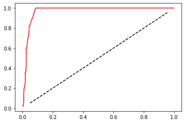
Now we have drawn the ROC curve. How do we understand this curve? Let's Recall that the fundamental purpose of establishing ROC curve is to find the balance between Recall and fpr, so that we can measure how the model will hurt most classes when it tries to capture a few classes. The abscissa is fpr, which represents the ability of the model to judge most classes incorrectly, and the ordinate Recall represents the ability of the model to capture a few classes. Therefore, the ROC curve represents how fpr increases with the continuous increase of Recall. We hope that with the continuous improvement of Recall, the slower the FPR increases, the better. This shows that we can catch a few classes as efficiently as possible without misjudging many classes. So what we want to see is that the ordinate rises rapidly, The abscissa grows slowly, that is, an arc at the top left of the whole image. This means that the effect of the model is very good and has a good ability to capture a few classes.
The dotted line in the middle indicates that when recall increases by 1%, our FPR also increases by 1%, that is, every time we capture a few classes, a majority class will be judged wrong. In this case, the effect of the model is not good. The result of capturing a few classes by this model will cause many classes to be injured by mistake, thus increasing our cost. ROC curves are usually convex. For a convex ROC curve, the closer the curve is to the upper left corner, the better, and the lower the curve is, the worse. If the curve is below the dotted line, it proves that the model is completely unusable. But it may also be a concave ROC curve. For a concave ROC curve, the closer it is to the lower right corner, the better. The concave curve represents that the prediction result of the model is completely opposite to the real situation, which is not very bad. As long as we manually reverse the result of the model, we can get an upper left arc. The worst thing is, whether the curve is concave or convex, the curve is in the middle of the image and very close to the dotted line, so there is nothing we can do with it.
Well, now that we have this curve, we do know that the effect of the model is good. But it is still very ambiguous. Are there any specific figures to help us understand the effect of ROC curve and model? Indeed, this number is called AUC area, which represents the area below the ROC curve. The larger the area, the closer the ROC curve is to the upper left corner, the better the model. The calculation of AUC area is cumbersome, so we use sklearn to help us. Next, let's look at how to draw our ROC curve and find out our AUC area in sklearn.
Using ROC curve to find the best threshold
In sklearn, we help us calculate the abscissa false positive rate FPR, ordinate Recall and the corresponding threshold class sklearn.metrics.roc of ROC curve_ curve. At the same time, the class sklearn.metrics.roc helps us calculate the AUC area_ auc_ score. In some older versions of sklearn, we use the class sklearn.metrics.auc to calculate the AUC area, but this class will be abandoned in version 0.22. Therefore, it is recommended that everyone use roc_auc_score, let's take a look at our two classes:
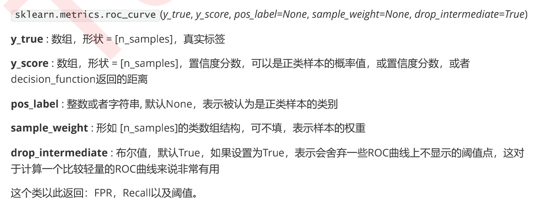
Confidence, probability as y_score is OK
from sklearn.metrics import roc_curve

FPR, recall, thresholds = roc_curve(y,clf_proba.decision_function(X), pos_label=1)

print(FPR)
print(recall)
print(thresholds)
result:
[0.    0.    0.006 0.006 0.008 0.008 0.01  0.01  0.014 0.014 0.018 0.018
 0.022 0.022 0.024 0.024 0.028 0.028 0.03  0.03  0.032 0.032 0.036 0.036
 0.04  0.04  0.042 0.042 0.044 0.044 0.05  0.05  0.054 0.054 0.058 0.058
 0.066 0.066 0.072 0.072 0.074 0.074 0.086 0.086 1.   ]

[0.   0.02 0.02 0.06 0.06 0.16 0.16 0.2  0.2  0.22 0.22 0.36 0.36 0.42
 0.42 0.6  0.6  0.62 0.62 0.64 0.64 0.68 0.68 0.7  0.7  0.74 0.74 0.76
 0.76 0.82 0.82 0.84 0.84 0.86 0.86 0.88 0.88 0.92 0.92 0.94 0.94 0.96
 0.96 1.   1.  ]

[  3.18236076   2.18236076   1.48676267   1.35964325   1.33920817
   1.14038015   1.13383091   1.00003406   0.85085628   0.84476439
   0.78571364   0.60568093   0.5389064    0.46718521   0.44396046
   0.03907036  -0.07011269  -0.10668727  -0.1258212   -0.13845693
  -0.14034183  -0.16790648  -0.2040958   -0.22137683  -0.24381463
  -0.26762451  -0.34446784  -0.3467975   -0.39182241  -0.40676459
  -0.4589064   -0.46310299  -0.49195707  -0.5088941   -0.53560561
  -0.55152081  -0.62628865  -0.67580418  -0.78127198  -0.79874442
  -0.88438995  -0.91257798  -1.01417607  -1.08601917 -10.31959605]
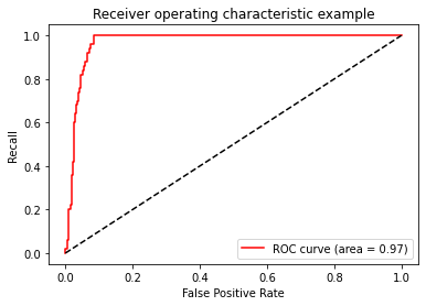
from sklearn.metrics import roc_auc_score as AUC
area = AUC(y,clf_proba.decision_function(X))
area
result:
0.9696400000000001
plt.figure()
plt.plot(FPR, recall, color='red',label='ROC curve (area = %0.2f)' % area)
plt.plot([0, 1], [0, 1], color='black', linestyle='--')
plt.xlim([-0.05, 1.05])
plt.ylim([-0.05, 1.05])
plt.xlabel('False Positive Rate')
plt.ylabel('Recall')
plt.title('Receiver operating characteristic example')
plt.legend(loc="lower right")
plt.show()
result:
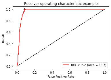
Now, with the ROC curve, we understand the classification effectiveness of the model and the effectiveness in the face of sample imbalance. How can we solve our best threshold? We want to know what kind of situation our model is the best. Back to our understanding of the ROC curve: the ROC curve reflects how the FPR changes when recall increases, that is, when the ability of the model to capture a small number of classes becomes stronger, it will hurt most classes by mistake. Our hope is that when the ability of capturing a few classes becomes stronger, the model will try not to hurt most classes by mistake, that is, with the increase of recall, fpr will increase The smaller the size, the better. Therefore, the most important point we hope to find is the point where the gap between recall and fpr is the largest. This point is also called the Jordan index.
maxindex = (recall - FPR).tolist().index(max(recall - FPR))
print(thresholds[maxindex])

#We can see where this point is in the image
plt.scatter(FPR[maxindex],recall[maxindex],c="black",s=30)

#Put the above code into this Code:
plt.figure()
plt.plot(FPR, recall, color='red',label='ROC curve (area = %0.2f)' % area)
plt.plot([0, 1], [0, 1], color='black', linestyle='--')
plt.scatter(FPR[maxindex],recall[maxindex],c="black",s=30)
plt.xlim([-0.05, 1.05])
plt.ylim([-0.05, 1.05])
plt.xlabel('False Positive Rate')
plt.ylabel('Recall')
plt.title('Receiver operating characteristic example')
plt.legend(loc="lower right")
result:
The best threshold is thus selected, because now we use decision_function to draw ROC curve, so the best threshold we choose is actually the best distance. If we use probability, the best threshold we choose will make a probability value. As long as we make the points above the distance / probability positive and the points below the distance / probability negative, the model is the best: that is, it can capture a few classes and try not to hurt most classes. The overall accuracy and capture of a few classes are guaranteed.
From the point of view of the optimal threshold point found, this point is actually the point closest to the upper left corner of the image, the point farthest from the dotted line in the middle, and also the turning point of the ROC curve. If there is no time for calculation, or when the abscissa is clear, we can observe the turning point to find our best threshold.
So far, the SVC model evaluation indicators have been introduced. However, the sample imbalance problem of SVC can still be explored. In addition, we can also use KS curve or yield curve (pro fi t) chart) to select our threshold, which is similar to ROC curve. If you have spare power, you can study it yourself. Model evaluation indicators, there are many profound places.