This paper mainly analyzes the Yansai 2015D problem, applies the optimization model, and involves the genetic algorithm and simulated annealing algorithm in modern optimization algorithms.
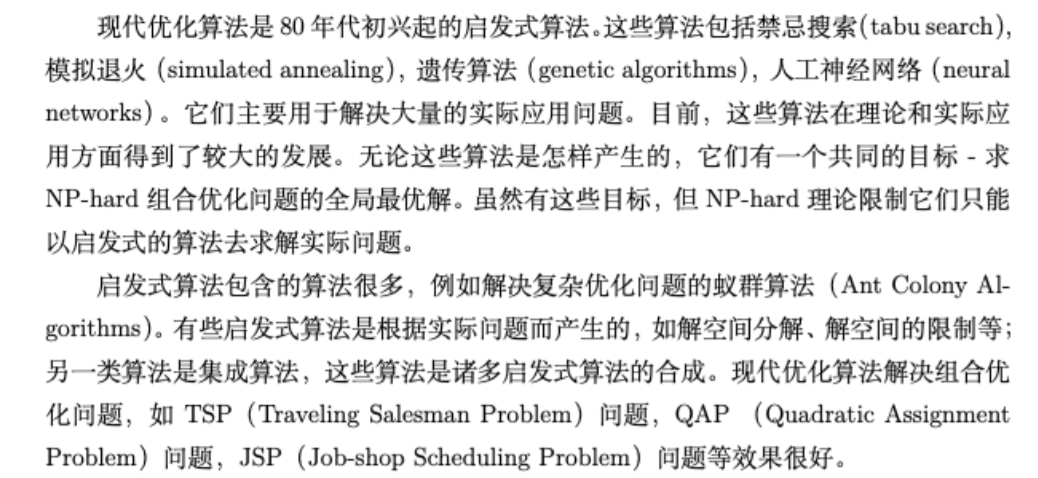
Modern optimization algorithms (genetic algorithm, simulated annealing algorithm, ant colony algorithm and tabu search algorithm) are very powerful, but they are more difficult than other algorithms such as grey prediction. For mathematical modeling, it is enough to master genetic algorithm and simulated annealing. Even if it is not enough, learning these two algorithms well, ant colony algorithm and tabu search will be easier to understand.
1 list of topics (2015D)
Problem 1: optimal control of energy-saving operation of single train
- Please establish a mathematical model to calculate the speed distance curve and find a train from A 6 A_6 A6 station departure and arrival A 7 A_7 The speed distance curve of the most energy-saving operation of A7} station, in which the operation time between two stations is 110 seconds. See the documents "train parameters. xlsx" and "line parameters. xlsx" for train parameters and line parameters.
- Please establish a new mathematical model to calculate the speed distance curve and find a train from A 6 A_6 A6 station departure and arrival A 8 A_8 A8. Speed distance curve of the most energy-efficient operation of the station, in which the train is required to A 7 A_7 A7. Stop at the station for 45 seconds, A 6 A_6 A6 station and A 8 A_8 A8. The total operation time between stations is specified as 220 seconds (excluding dwell time). For train parameters and line parameters, see the documents "train parameters. xlsx" and "line parameters. xlsx".
Problem 2: optimal control of multi train energy-saving operation
When 100 trains run at intervals H = { h 1 , ... , h 9 9 } H=\{ h_1,...,h_99\} H={h1,..., h9} from A 1 A_1 A1} station departure, tracking operation, passing by in turn A 2 A_2 A2, A 3 A_3 A3,... Arrive A 14 A_{14} A14 ¢ stop at each station at least in the middle D min D_{\min} Dmin , seconds, max D max D_{\max} Dmax = seconds. interval H H The variation range of each component of H is H min H_{\min} Hmin seconds to H max H_{\max} Hmax = seconds. Please establish the optimization model and find the interval to minimize the total energy consumption of all trains H H H. The interval between the departure time of the first train and the departure time of the last train is required to be T 0 = 63900 T_0=63900 T0 = 63900 seconds and from A 1 A_1 A1 , station to A 14 A_{14} A14 # the total operation time of the station remains unchanged, which is 2086s (including station dwell time). Assuming that all trains are in the same power supply section, the line parameters between stations are detailed in the documents "train parameters. xlsx" and "line parameters. xlsx".
Problem 3: optimal control of train operation after delay
Then ask, if the train i i i at the station A j A_j Aj delay D T j i DT_j^i DTji (10 seconds) departure, please establish the control model and find out the train operation curve with the least energy consumption during the recovery period on the premise of ensuring safety. If the arrival and departure time of the train at each station is allowed to be no more than 10 seconds ahead of the original time, how to adjust the control scheme of the second question according to the above statistical data?
2 Genetic Algorithm (GA)
2.1 theoretical basis
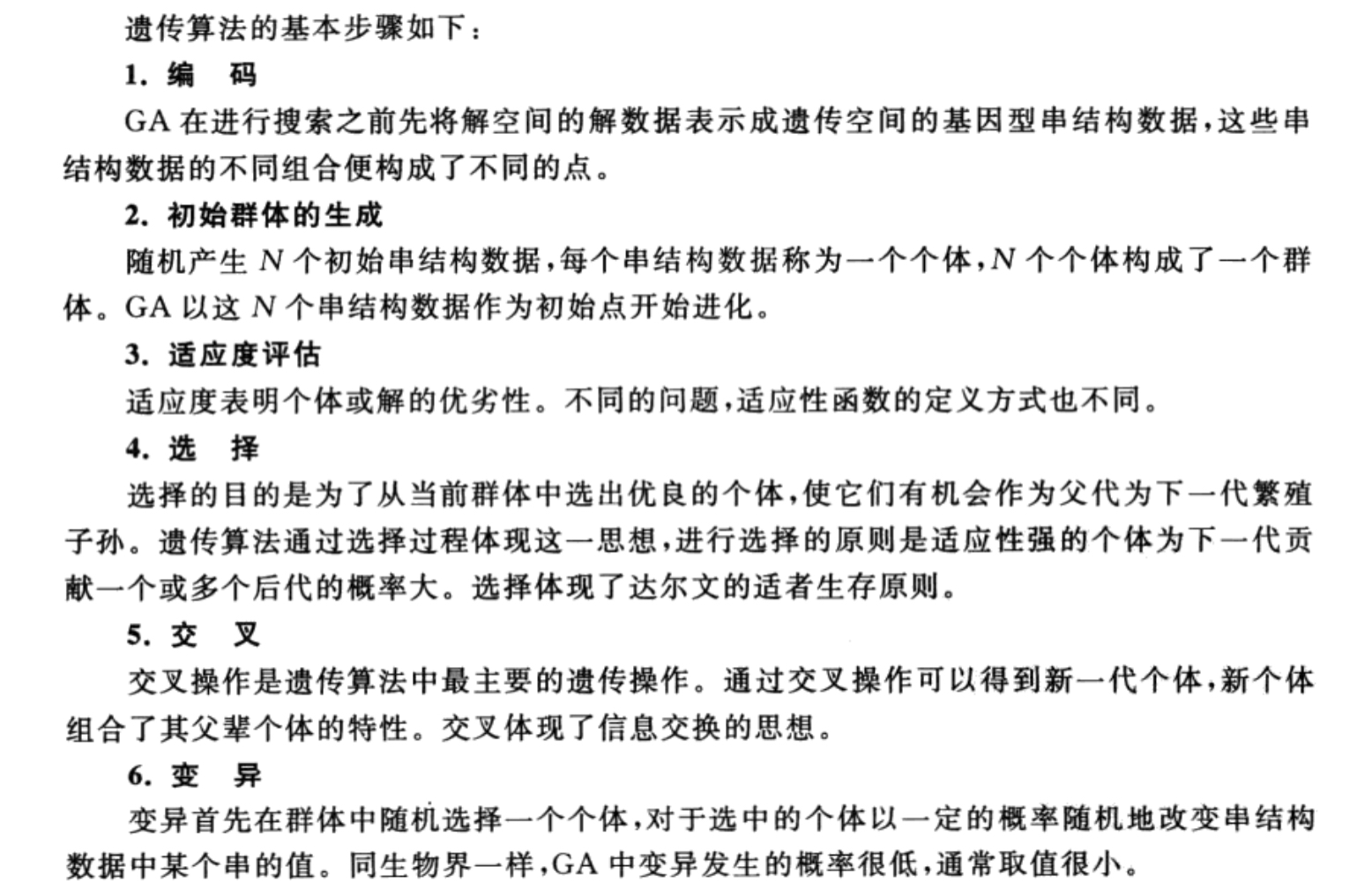
- Basic principle: follow the evolution law of "natural selection and survival of the fittest" in the biological world. Genetic algorithm encodes the problem parameters into chromosomes, and then uses iterative methods to carry out selection, crossover and mutation operations to exchange chromosome information in the population, and finally generate chromosomes that meet the optimization objectives
- General structure: gene = > chromosome (gene string / genotype individuals)) = > population
Of which:
① Chromosome: data or array (usually one-dimensional string structure data) to represent the value of the corresponding gene at each position on the string
② population size: the number of individuals in a population
③ fitness: the degree of adaptation of each individual to the environment - Basic steps:
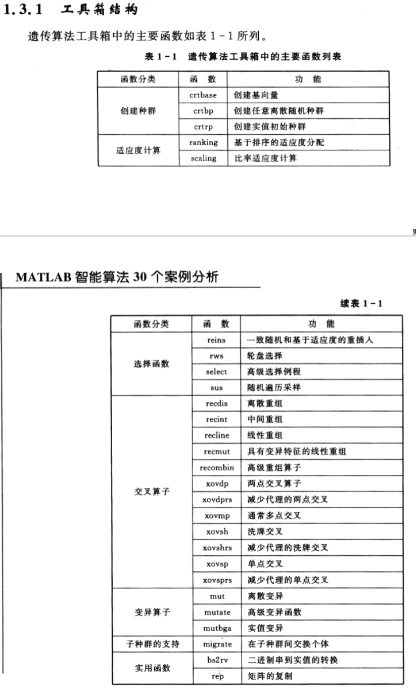
2.2 detailed explanation and application of toolbox
2.2.1 Sheffield genetic toolbox
- Download link: MATLAB Sheffield genetic algorithm toolbox
- Toolbox main functions
Example: using genetic algorithm to find function f ( x ) = s i n ( 10 π x ) x f(x)=\frac{sin(10\pi x)}{x} f(x)=xsin(10 π x) at [ 1 , 2 ] [1,2] Minimum value on [1,2].
clc
clear all
close all

%%Draw a function diagram
figure(1);
hold on;
lb=1;ub=2;%Range of function arguments[1,2]
fplot(@(X) sin(10*pi*X)./X,[lb,ub]);%Draw the function curve
xlabel('independent variable/X')
ylabel('Function quantity/Y')

%%Defining genetic algorithm parameters
NIND=40;%Population size
MAXGEN=20;%Maximum genetic algebra
PRECI=20;%Individual length
GGAP=0.95;%generation gap
px=0.7;%Crossover probability
pm=0.01;%Variation probability
trace=zeros(2,MAXGEN);%Initial value of optimization result
FieldD=[PRECI;lb;ub;1;0;1;1];%Area descriptor
Chrom=crtbp(NIND,PRECI);%Create any discrete random population

%%optimization
gen=0;%Generation counter
X=bs2rv(Chrom,FieldD);%Initial population binary to decimal conversion
ObjV=sin(10*pi*X)./X;%Calculate objective function value
while gen<MAXGEN
    FitnV=ranking(ObjV);%Allocation fitness
    SelCh=select('sus',Chrom,FitnV,GGAP);%choice
    SelCh=recombin('xovsp',SelCh,px);%recombination
    SelCh=mut(SelCh,pm);%variation
    X=bs2rv(SelCh,FieldD);%Decimal conversion of descendant individuals
    ObjVSel=sin(10*pi*X)./X;%Calculate the objective function value of the offspring
    [Chrom,ObjV]=reins(Chrom,SelCh,1,1,ObjV,ObjVSel);%Insert the progeny to the parent again to get the new population
    X=bs2rv(Chrom,FieldD);
    gen=gen+1;%Generation counter increase
    %Obtain the optimal solution of each generation and its sequence number, Y Is the optimal solution, I Mark individual
    [Y,I]=min(ObjV);
    trace(1,gen)=X(I);%Note the optimal value of each generation
    trace(2,gen)=Y;%Note the optimal value of each generation
end
plot(trace(1,:),trace(2,:),'bo');%Draw the best of each generation
grid on;
plot(X,ObjV,'b*')%Draw the last generation of the population
hold off

%%Draw an evolution map
figure(2);
plot(1:MAXGEN,trace(2,:));
grid on;
xlabel('Genetic algebra')
ylabel('Change of solution')
title('evolutionary process ')
bestY=trace(2,end);
bestX=trace(1,end);
fprintf(['Optimal solution:\nX=',num2str(bestX),' \nY=',num2str(bestY),'\n'])
Example: using genetic algorithm to find function f ( x , y ) = x cos ( 2 π y ) + y sin ( 2 π x ) , x ∈ [ − 2 , 2 ] , y ∈ [ − 2 , 2 ] f(x,y)=x\cos (2\pi y)+y \sin (2\pi x),\ x\in [-2,2],\ y\in [-2,2] f(x,y)=xcos(2πy)+ysin(2πx), x∈[−2,2], The maximum value of Y ∈ [− 2,2].
clc
clear all
close all
%%Draw a function diagram
figure(1);
lbx=-2;ubx=2;%Function argument x Scope of[-2,2]
lby=-2;uby=2;%Function argument y Scope of[-2,2]
fmesh(@(x,y) y.*sin(2*pi*x)+x.*cos(2*pi*y),[lbx,ubx,lby,uby]);%Draw the function curve
hold on;
%%Defining genetic algorithm parameters
NIND=40;%Population size
MAXGEN=50;%Maximum genetic algebra
PRECI=20;%Individual length
GGAP=0.95;%generation gap
px=0.7;%Crossover probability
pm=0.01;%Variation probability
trace=zeros(3,MAXGEN);%Initial value of optimization result
FieldD=[PRECI PRECI;lbx lby;ubx uby;1 1;0 0;1 1;1 1];%Area descriptor
Chrom=crtbp(NIND,PRECI*2);%Create any discrete random population
%%optimization
gen=0;%Generation counter
XY=bs2rv(Chrom,FieldD);%Initial population binary to decimal conversion
X=XY(:,1);Y=XY(:,2);
ObjV=Y.*sin(2*pi*X)+X.*cos(2*pi*Y);%Calculate objective function value
while gen<MAXGEN
FitnV=ranking(-ObjV);%Allocation fitness
SelCh=select('sus',Chrom,FitnV,GGAP);%choice
SelCh=recombin('xovsp',SelCh,px);%recombination
SelCh=mut(SelCh,pm);%variation
XY=bs2rv(SelCh,FieldD);%Decimal conversion of descendant individuals
X=XY(:,1);Y=XY(:,2);
ObjVSel=Y.*sin(2*pi*X)+X.*cos(2*pi*Y);%Calculate the objective function value of the offspring
[Chrom,ObjV]=reins(Chrom,SelCh,1,1,ObjV,ObjVSel);%Insert the progeny to the parent again to get the new population
XY=bs2rv(Chrom,FieldD);
gen=gen+1;%Generation counter increase
%Obtain the optimal solution of each generation and its sequence number, Y Is the optimal solution, I Mark individual
[Y,I]=max(ObjV);
trace(1:2,gen)=XY(I,:);%Note the optimal value of each generation
trace(3,gen)=Y;%Note the optimal value of each generation
end
plot3(trace(1,:),trace(2,:),trace(3,:),'bo');%Draw the best of each generation
grid on;
plot3(XY(:,1),XY(:,2),ObjV,'b*')%Draw the last generation of the population
hold off
%%Draw an evolution map
figure(2);
plot(1:MAXGEN,trace(3,:));
grid on;
xlabel('Genetic algebra')
ylabel('Change of solution')
title('evolutionary process ')
bestZ=trace(3,end);
bestY=trace(2,end);
bestX=trace(1,end);
fprintf(['Optimal solution:\nX=',num2str(bestX),'\nY=',num2str(bestY),'\nZ=',num2str(bestZ),'\n'])```
🤔: The results are different every time. How to ensure the stability of the algorithm?
# 3 simulated annealing (SA)
## 3.1 theoretical basis
The idea of simulated annealing algorithm was first developed by Metropolis The starting point is based on the similarity between the annealing process of solid matter in physics and the general combinatorial optimization problem.
1. Physical annealing process
The physical annealing process consists of the following three parts:
(1)Heating process: the purpose is to enhance the thermal motion of particles and make them deviate from the equilibrium position. When the temperature is high enough, the solid will melt into liquid, so as to eliminate the original non-uniform state of the system
(2)Isothermal process: for a closed system that exchanges heat with the surrounding environment and the temperature remains unchanged, the spontaneous change of the system state is always in the direction of reducing the free energy. When the free energy reaches the minimum, the system reaches the equilibrium state
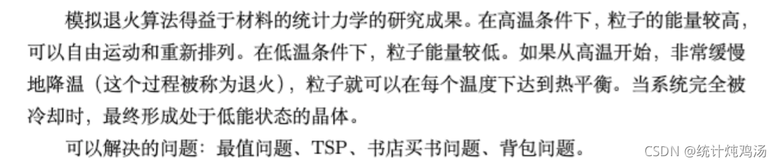
(3)Cooling process: the thermal motion of particles is weakened, the system energy is reduced, and the crystal structure is obtained
| physical process |Corresponding algorithm |
|--|--|
| Heating process| Set initial temperature|
|Isothermal process|Metropolis Sampling process|
|cooling process |Decrease of control parameters|
|Energy change|objective function |
|Lowest energy state|Optimal solution|
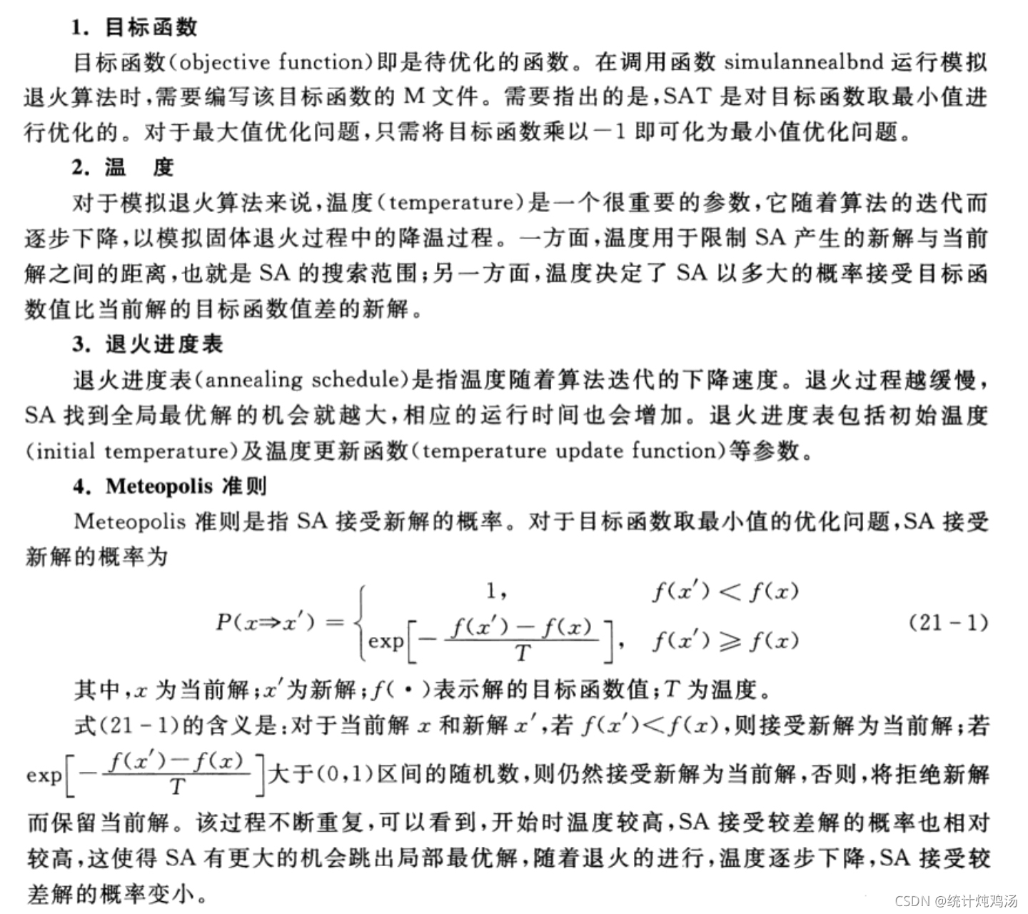
2. SA Key of algorithm—— Metropolis criterion
Metropolis The rule is SA The key to the convergence of the algorithm to the global optimal solution, Metropolis The criterion accepts the deteriorating solution with a certain probability, which makes the algorithm jump away from the trap of local optimal solution.
3. advantage
Simulated annealing algorithm can be used to solve different nonlinear problems. For the optimization of non differentiable or even discontinuous functions, it can obtain the global optimization solution with high probability. The algorithm also has strong robustness, global convergence, implicit parallelism and wide adaptability, and can deal with different types of optimization design variables (discrete, continuous and mixed), No auxiliary information is required, and there are no requirements for objective functions and constraints. utilize Metropolis The algorithm and properly control the temperature drop process have strong competitiveness in the optimization problem.
4. Implementation process
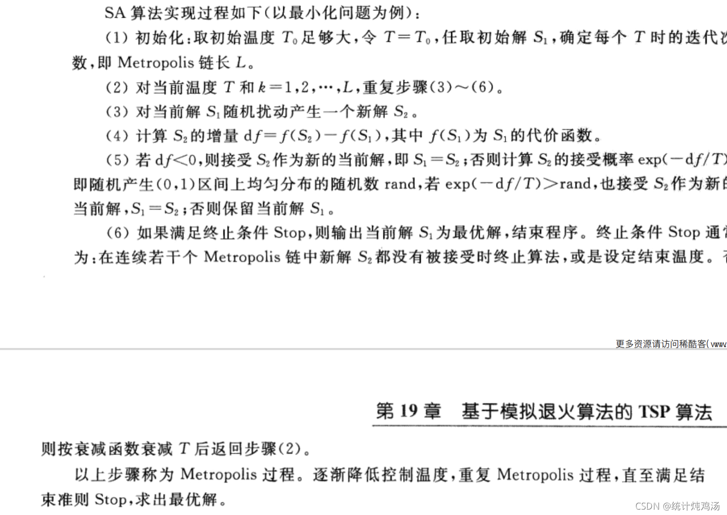
## 3.2 toolbox explanation and Application
### 3.2.1 simulated annealing algorithm toolbox
MATLAB Optimization toolbox is included in( Global Optimization Toolbox R2021a Author: MathWorks),It contains the simulated annealing algorithm part, which we call the simulated annealing algorithm toolbox( Simululated Annealing Toolbox,SAT).
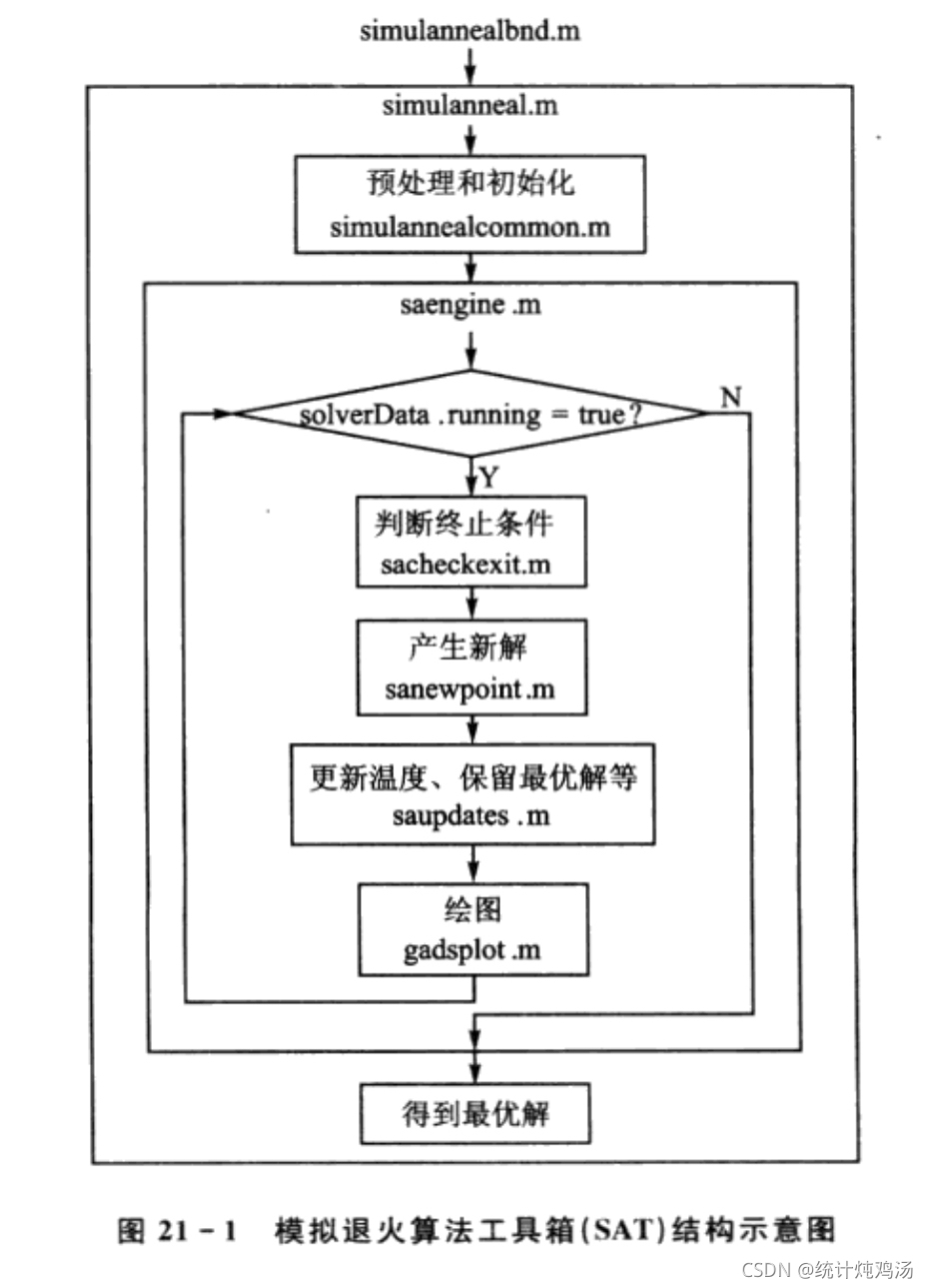
As you can see, in the iteration loop, the function sanewpoint Sum function saupdates Is the key function.
### 3.2.2 basic concepts
# 4 thesis analysis
## 3.1 genetic algorithm

## 3.2 simulated annealing algorithm
! [insert picture description here]( https://img-blog.csdnimg.cn/8033351e7ee24a37bcac914ad639f951.png#pic_center)