6.2.1 data set introduction
The data used in this OCR experiment is based on Task 4.3:Word Recognition in icdar2015 incident scene text. This is a word recognition task. Remove some pictures to simplify the difficulty of this experiment.
The data set contains many text areas in natural scene images. The training set in the original data contains 4468 images and the test set contains 2077 images. They are cut out from the original large image according to the bounding box of the text area, and the text in the image is basically in the center of the picture.
The dataset contains folders containing images and corresponding label files, which are divided into train and test. Similar forms such as word_1.png, "join", i.e. word_ 1. The image result of PNG is the English word join.
In order to simplify the recognition difficulty of subsequent experiments, the data set provided roughly filters the vertically arranged images of characters with an aspect ratio > 1.5, so it is slightly different from the original data set of ICDAR2015.
6.2.2 data analysis and character mapping relationship construction
Before the experiment, simply analyze the data to understand the characteristics of the data.
The specific work is: tag character statistics (which characters are there and how many times each character appears), longest tag length statistics, image size analysis, etc. are carried out on the data, and the mapping relationship file lbl2id of character tags is constructed_ map.txt.
preparation
import os
import cv2

#Data set root directory, please download the data to this location
base_data_dir='./ICDAR_2015'

#Training data set and validation data
train_img_dir=os.path.join(base_data_dir,'train')
valid_img_dir=os.path.join(base_data_dir,'valid')
#Training set and validation set label file paths
train_lbl_path=os.path.join(base_data_dir,'train_gt.txt')
valid_lbl_path=os.path.join(base_data_dir,'valid_gt.txt')
#The intermediate file storage path stores the mapping relationship between label characters and their IDs
lbl2id_map_path=os.path.join(base_data_dir,'lbl2id_map.txt')
1. Statistics of the longest characters of the label
First, count the number of characters contained in the longest label in the data set. Here, count the longest label in both the training set and the verification set to get the characters contained in the longest label.
def statistics_max_len_label(lbl_path):
'''
Count the longest in the tag file label Number of characters contained
lbl_path:txt Label file path
'''
max_len=-1
with open(lbl_path,'r') as reader:
    for line in reader:
        items=line.rstrip().split(',')
        # img_name=items[0] #Extract image name
        lbl_str=items[1].strip()[1:-1] #Extract the label and remove the quotation mark "" from the label
        lbl_len=len(lbl_str)
        max_len=max_len if max_len>lbl_len else lbl_len
return max_len

train_max_label_len=statistics_max_len_label(train_lbl_path) #Longest training set label
valid_max_label_len=statistics_max_len_label(valid_lbl_path) #Verification set longest label
max_label_len=max(train_max_label_len,valid_max_label_len) #The longest label in the whole dataset
print(f"The data set contains the most characters label Count Reg{max_label_len}")
The longest label in the dataset contains 21 characters, which will provide a reference for the setting of time steps when the transformer model is built later.
2. Statistics of characters contained in labels
View all characters that have appeared in the dataset
def statistics_label_cnt(lbl_path,lbl_cnt_map):
'''
Statistics tag file label What characters are included and how many times they appear
lbl_path:Path to label file
lbl_cnt_map:A dictionary that records the number of occurrences of characters in a label
'''
with open(lbl_path,'r') as reader:
    for line in reader:
        items=line.rstrip().split(',')
        #img_name=items[0]
        lbl_str=items[1].strip()[1:-1] #Extract the label and remove the double quotation mark "" in the label
        for lbl in lbl_str:
            if lbl not in lbl_cnt_map.keys():
                lbl_cnt_map[lbl]=1
            else:
                lbl_cnt_map[lbl] +=1

lbl_cnt_map=dict() #A dictionary used to store the number of occurrences of characters
statistics_label_cnt(train_lbl_path,lbl_cnt_map)#Statistics of character occurrences in training set
print("Training concentration label Characters appearing in:")
print(lbl_cnt_map)
statistics_label_cnt(valid_lbl_path,lbl_cnt_map)#Statistics of character occurrences in training set and verification set
print("Training set+Validation set label Characters appearing in:")
print(lbl_cnt_map)
lbl_cnt_map is a statistical Dictionary of the number of occurrences of characters. It will also be used to establish the mapping relationship between characters and their IDs.
From the statistical results of the data set, the test set contains characters that have not appeared in the training set. The number of such cases is small, so it should not be a problem, so no additional processing is performed on the data set here (but it is necessary to consciously check whether there is difference between the training set and the test set).
3. Construction of mapping dictionary between char and id
In the OCR task of this paper, it is necessary to predict each character in the picture. In order to achieve this purpose, we first need to establish a mapping relationship between a character and its id, and convert the text information into digital information that can be read by the model. This step is similar to establishing a corpus in NLP.
When building a mapping relationship, in addition to recording the characters appearing in all label files, three special characters need to be initialized to represent a sentence start character, sentence end character and padding identifier respectively.
Build the mapping relationship between char and ID. finally, the mapping relationship will be saved in lbl2id_ In the map.txt file
#Mapping between characters -- id in label construction
print("structure label Chinese character--id Mapping between:")
lbl2id_map=dict()
#Initialize three special characters
lbl2id_map['☯']=0 #padding identifier
lbl2id_map['■']=1 #Sentence starter
lbl2id_map['□']=2 #Sentence Terminator
#Generate id mapping relationships for the remaining characters
cur_id=3
for lbl in lbl_cnt_map.keys():
    lbl2id_map[lbl]=cur_id
    cur_id+=1
#Save the mapping between characters -- id to txt file
with open(lbl2id_map_path,'w',encoding='utf_8_sig') as writer:#The parameter encoding is optional. Some devices do not default to UTF_ eight
   for lbl in lbl2id_map.keys():
       cur_id=lbl2id_map[lbl]
       print(lbl,cur_id)
       line=lbl+'\t'+str(cur_id)+'\n'
       writer.write(line)
To establish a relationship mapping dictionary, you can read the file containing the mapping relationship txt to build a character to id and id to character mapping dictionary. This serves the subsequent transformer training process to facilitate the fast conversion of character relationships.
def load_lbl2id_map(lbl2id_map):
'''
Read character-id Of mapping relationship records txt File and return lbl->id and id->lbl Mapping dictionary
lbl2id_map_path:character-id Of mapping relationship records txt File path
'''
    lbl2id_map=dict()
    id2lbl_map=dict()
    with open(lbl2id_map_path,'r') as reader:
        for line in reader:
            items=line.rstrip().split('\t')
            label=items[0]
            cur_id=int(items[1])
            lbl2id_map[label]=cur_id
            id2lbl_map[cur_id]=label
    return lbl2id_map,id2lbl_map
4. Data set image size analysis
When carrying out tasks such as image classification and detection, we often check the size distribution of the image, and then determine the appropriate image preprocessing method. For example, when carrying out target detection, we will count the size of the bounding box of the image size, analyze the aspect ratio, and then select the appropriate image clipping strategy and the appropriate initial anchor strategy.
Analyze the image width, height and aspect ratio to understand the characteristics of the data
#Analyze dataset picture size
print("Analysis dataset picture size:")

#Initialization parameters
min_h=1e10
min_W=1e10
max_h=-1
max_w=-1
min_ratio=1e10
max_ratio=0
#Traverse the dataset to calculate size information
for img_name in os.listdir(train_img_dir):
    img_path=os.path.join(train_img_dir,img_name)
    img=cv2.imread(img_path) #Read picture
    h,w=img.shape[:2] #Extract image height and width information
    ratio=w/h #Aspect ratio
    min_h=min_h if min_h <=h else h #Minimum picture height
    max_h=max_h if max_h >=h else h #Maximum picture height
    min_w=min_w if min_w<=w else w #Minimum picture width
    max_w=max_w if max_w >=w else w #Maximum picture width
    min_ratio=min_ratio if min_ratio <= ratio else ratio #Minimum aspect ratio
    max_ratio=max_ratio if max_ratio >= ratio else ratio #Maximum aspect ratio
#Output information
print('min_h',min_h)
print('max_h',max_h)
print('min_w',min_w)
print('max_w',max_w)
print('min_ratio',min_ratio)
print('max_ratio',max_ratio)
Most of the pictures are long strips lying down, and the maximum aspect ratio is > 8. It can be seen that there are extremely slender pictures.
6.2.3 how to introduce transformer into OCR
Why can transformer solve OCR problems?
- transformer is widely used in NLP field and can solve the problem of sequence to sequence class such as machine translation.
- OCR recognition task, which wants to identify the contents in the figure, can also be regarded as a sequence to sequence task in essence, but the input sequence information is represented in the form of pictures.
- From the perspective of treating OCR problem as a sequence to sequence prediction problem, it seems to be a very natural and smooth idea to use transformer to solve OCR problem. The remaining problem is how to construct image information into input similar to word embedding to meet the input requirements of transformer.
- Since the pictures to be predicted are long strips and the characters are basically arranged horizontally, we integrate the feature map along the horizontal direction, and each embedding obtained can be regarded as the feature of a slice in the vertical direction of the picture. Such feature sequence is handed over to the transformer, which uses its powerful attention ability to complete the prediction.
The model framework pipeline is shown in the figure:
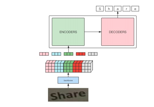
By observing the above figure, it can be found that the whole pipeline is basically the same as the process of training machine translation with transformer, and the difference is mainly due to the process of extracting image features with a CNN network as the backbone to obtain input embedding.
6.2.4 detailed explanation of training framework code
The related codes of training framework are implemented in ocr_by_transformer.py file
Let's start to explain the code step by step, mainly including the following parts:
- Build dataset - > image preprocessing, label processing, etc
- Model construction - > backbone + transformer
- model training
- Reasoning - > greedy decoding
1. Preparation
First, import the library to be used later
import os
import time
import copy
import numpy as np
from PIL import Image

#torch related package
import torch
import torch.nn as nn
from torch.autograd import Variable
import torchvision.models as models
import torchvision.transforms as transforms

#Import tool class package
from analysis_recognition_dataset import load_lbl2id_map,statistics_max_len_label
from transformer import *
from train_utils import *
Then set some basic parameters
base_data_dir='../../../dataset/ICDAR_2015' #Data set root directory, please download the data to this location
device=torch.device("cuda") #'cpu' or 'cuda'
nrof_epochs=1500 #Number of iterations, 1500, revised according to requirements
batch_size=64  #Batch size, 64, corrected as required
model_save_path='./log/ex1_ocr_model.pth'
Read the mapping dictionary between the character and its id in the image label, which needs to be used for subsequent Dataset creation.
#Read the label ID mapping record file
lbl2id_map_pat=os.path.join(base_data_dir,'lbl2id_map.txt')
lbl2id_map,id2lbl_map=load_lbl2id_map(lbl2id_map_path)

#Statistics on the number of characters in all label s in the dataset that contain the most characters. The data set construction gt(ground truth) information needs to be used
train_lbl_path=os.path.join(base_data_dir,'train_gt.txt')
valid_lbl_path=os.path.join(base_data_dir,'valid_gt.txt')
train_max_label_len=statistics_max_len_label(train_lbl_path)
valid_max_label_len=statistics_max_len_label(valid_lbl_path)
#The case with the largest number of characters in the dataset is used as the sequence of gt_ len
sequence_len=max(train_max_label_len,valid_max_label_len)
2. Dataset construction
Let's introduce the related contents of Dataset construction. First, it's reasonable to think about how to preprocess images.
Picture preprocessing scheme
Suppose the picture size is [batch_size,3,
H
i
H_i
Hi,
W
i
W_i
Wi]
The size of the characteristic diagram after passing through the network is [batch_size,
C
f
C_f
Cf,
H
f
H_f
Hf,
W
f
W_f
Wf]
Based on the previous analysis of the data set, the pictures are basically horizontal long strips, and the image content is words composed of horizontally arranged characters. Then, the position of the same vertical slice in the picture space basically has only one character, so the vertical resolution does not need to be very large, so take
H
f
=
1
H_f=1
Hf = 1; the horizontal resolution needs to be larger. We need different embedding to encode the characteristics of different characters in the horizontal direction.
Here, we use the most classic resnet18 network as the backbone. Because its lower sampling multiple is 32 and the number of channel s in the last layer of characteristic graph is 512, then:
H
i
=
H
f
∗
32
=
32
H_i=H_f*32=32
Hi=Hf∗32=32
C
f
=
512
C_f=512
Cf=512
How to determine the width of the input picture? Here are two schemes, as shown in the figure below:
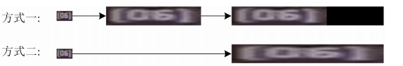
Method 1: set a fixed size, resize the image with its aspect ratio, and pad the empty area on the right;
Method 2: directly force the original image to resize to a preset fixed size.
Note: which scheme is better?
Here, the author chose method 1, because the aspect ratio of the picture is roughly proportional to the number of characters of words in the picture. If the aspect ratio of the original picture is maintained during preprocessing, the range of each pixel on the feature map corresponding to the character area on the original image is basically stable, which may have a better prediction effect.
Here's another detail. If you look at the above figure, you will find that each area with width: height = 1:1 is basically distributed with 2-3 characters. Therefore, in actual operation, we did not strictly keep the width height ratio unchanged, but increased the width height ratio by 3 times, that is, first lengthen the width of the original image to 3 times, then maintain the width height ratio and resize the height to 32.
Note: it is suggested to stop and think again. Why is this detail just now?
The purpose of this is to make each character on the picture have at least one pixel on the feature map corresponding to it, rather than one pixel on the wide dimension of the feature map, and encode the information of multiple characters in the original image. I think this will bring unnecessary difficulties to the prediction of transformer.
The resize scheme is determined,
W
i
W_i
What is the specific setting of Wi? Combined with the two important indicators we analyzed in the data set earlier, the longest character in the data set label is 21 and the longest aspect ratio is 8.6. We set the final aspect ratio to 24:1. Therefore, we summarize the settings of various parameters:
H
i
=
H
f
∗
32
=
32
H_i=H_f*32=32
Hi=Hf∗32=32
W
i
=
24
∗
H
i
=
768
W_i=24*H_i=768
Wi=24∗Hi=768
C
f
=
512
,
H
f
=
1
,
W
f
=
24
C_f=512,H_f=1,W_f=24
Cf=512,Hf=1,Wf=24
Image preprocessing
#Image preprocessing
#load img
img=Image.open(img_path).convert('RGB')
#Zoom the picture approximately equally
#Reduce the height to 32 and the width to equal scale, but divide by 32
w,h=img.size
ratio=round((w/h)*3) #Lengthen the width three times and round it
if ratio==0:
    ratio = 1
if ratio>self.max_ratio:
    ratio=self.max_ratio
h_new=32
w_new=h_new*ratio
img_resize=img.resize((w_new,h_new)),Image.BILINEAR)

#padding the right half of the picture so that the width / height ratio is fixed = self.max_ratio
img_padd=Image.new('RGB',(32*self.max_ratio,32),(0,0,0))
img_padd.paste(img_resize,(0,0))
Image augmentation
Image enlargement is not the key point. Here, in addition to the above resize scheme, we only perform conventional random color transformation and normalization on the image.
Complete code for Dataset construction
class Recognition_Dataset(object):
   def __init__(self,dataset_root_dir,lbl2id_map,sequence_len,max_ration,phase='train',pad=0):
   if phase == 'train':
     self.img_dir=os.path.join(base_data_dir,'train')
     self.lbl_path=os.path.join(base_data_dir,'train_gt.txt')
   else:
     self.img_dir=os.path.join(base_data_dir,'valid')
     self.lbl_path=os.path.join(base_data_dir,'valid_gt.txt')
   self.lbl2id_map=lbl2id_map
   self.pad=pad #The id of the padding identifier. The default is 0
   self.sequence_len=sequence_len #Sequence length
   self.max_ratio=max_ratio*3 #Lengthen the width by 3 times

   self.imgs_list=[]
   self.lbls_list=[]
   with open(self.lbl_path,'r') as reader:
      for line in reader:
         items=line.rstrip().split(',')
         img_name=items[0]
         lbl_str=items[1].strip()[1:-1]

   #Define random color transformations
   self.color_trans=transforms.ColorJitter(0.1,0.1,0.1)
   #Define Normalize
   self.trans_Normalize=transforms.Compose([
       transforms.ToTensor(),
       transforms.Normalize([0.485,0.456,0.406],[0.229,0.224,0.225])])

   def __getitem__(self,index):
   '''
   Get corresponding index Images and ground truth label,And data enhancement as appropriate
   '''
   img_name=self.imgs_list[index]
   img_path=os.path.join(self.img_dir,img_name)
   lbl_str=self.lbls_list[index]

   #------------------------
   #Image preprocessing
   #------------------------
   #load image
   img=Image.open(img_path).convert('RGB')

   #Zoom the picture approximately equally
   #Reduce the height to 32 and the width to equal scale, but divide by 32
   w,h=img.size
   ratio=round((w/h)*3) #Lengthen the width three times and round it
   if ratio ==0:
       ratio=1
   if ratio > self.max_ratio:
       ratio=self.max_ratio
   h_new=32
   W_new=h_new*ratio
   img_resize=img.resize((w_new,h_new),Image.BILINEAR)

   #padding the right half of the picture so that the width / height ratio is fixed = self.max_ratio
   img_padd=Image.new("RGB",(32*self.max_ratio,32),(0,0,0))
   img_padd.paste(img_resieze,(0,0))

   #Random color transformation
   img_input=self.color_trans(img_padd)
   #Normalize
   img_input=self.trans_Normalize(img_input)

   #---------------------
   #label processing
   #---------------------

   #Construct mask of encoder
   encode_mask=[1]*ratio+[0]*(self.max_ratio-ratio)
   encode_mask=torch.tensor(encode_mask)
   encode_mask=(encode_mask !=0).unsqueeze(0)
   #Construct ground truth label
   gt=[]
   gt.append(1) #Add the sentence start character first
   for lbl in lbl_str:
       gt.append(self.lbl2id_map[lbl])
   gt.append(2)
   for i in range(len(lbl_str),self.sequence_len):
   #Except for the start and end characters, the length of lbl is sequence_len, and the remaining padding
       gt.append(0)
   #Truncate to the preset maximum sequence length
   gt=gt[:self.sequence_len+2]

   #Input of decoder
   decode_in=gt[:-1]
   decode_in=torch.tensor(decode_in)
   #Output of decoder
   decode_out=gt[1:]
   decode_out=torch.tensor(decode_out)
   #mask of decoder
   decode_mask=self.make_std_mask(decode_in,self.pad)
   #Number of valid tokens
   ntokens=(decode_out !=self.pad).data.sum()
   return img_input,encode_mask,decode_in,decode_out,decode_mask,ntokens

   @staticmethod
   def make_std_mask(tgt,pad):
   """
   Create a mask to hide padding and future words.
   padd and future words All in mask 0 in
   """
       tgt_mask=(tgt != pad)
       tgt_mask=tgt_mask & Variable(subsequent_mask(tgt.size(-1)).type_as(tgt_mask.data))
       tgt_mask=tgt_mask.squeeze(0) #When subsequence returns the shape of the value (1,N,N)
       return tgt_mask
   def __len__(self):
       return len(self.imgs_list)
encode_mask
Because we have adjusted the size of the image and padded the image according to the needs, and the padded position does not contain effective information, we need to construct the corresponding encode_mask according to the padding proportion, so that the transformer can ignore this meaningless area during calculation.
label processing
The prediction tags used in this experiment are basically the same as those used in machine translation model training, so there is little difference in processing methods.
In label processing, the characters in the label are converted into their corresponding id, and the start character is added at the beginning of the sentence, and the end character is added at the end of the sentence. When the length of sequence_len is not met, padding (0 filling) is performed at the remaining positions.
decode_mask
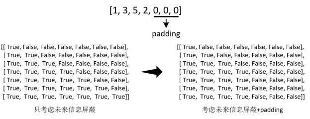
Generally, in the decoder, we will generate a mask in the form of upper triangular matrix according to the sequence_len of the label. Each line of the mask can control the current time_step. When the decoder is allowed to obtain only the character information before the current step, and it is prohibited to obtain the character information at the future time, which prevents cheating in model training.
The decode_mask is generated through a special function * * make_std_mask() *.
At the same time, it is also necessary to mask the padding part of the label of the decoder, so the decode_mask should also be written as False at the position corresponding to the label being padded.
The generated decode_mask is shown in the following figure:
Build a DataLoader for training
#Construct dataloader
max_ratio=8 #The maximum value of width / height during image preprocessing. If it does not exceed the guaranteed proportion, it will be forcibly compressed
train_dataset=Recognition_Dataset(base_data_dir,lbl2id_map,sequence_len,max_ratio,'train',pad=0)
valid_dataset=Recognition_Dataset(base_data_dir,lbl2id_map.sequence_len,max_ratio,'valid',pad=0)
#loader size info:
#--> img_input:[batch_size,c,h,w]-->[64,3,32,32*8*3]
#-->encode_mask:[batch_size,h/32,w/32]-->[64,1,24]#In this paper, the backbone adopts 32 times down sampling, so divide by 32
#-->decode_in:[bs,sequence_len-1]-->[64,20]
#-->decode_out:[bs,sequence_len-1]-->[64,20]
#-->decode_mask:[bs,sequence_len-1,sequence_len-1]-->[64,20,20]
#-->ntokens:[bs]-->[64]
train_loader=torch.utils.data.DataLoader(train_dataset,batch_size=batch_size,shuffle=True,num_workers=4)
valid_loader=torch.utils.data.DataLoader(valid_dataset,batch_size=batch_size,shuffle=False,num_workers=4)
3. Model construction
Code through make_ocr_model and OCR_ The encoderdecoder class completes the construction of the model structure.
From make_ ocr_ The model function looks like it first calls Resnet-18 pre trained in pytorch as the backbone to extract image features. It can also be adjusted to other networks according to its own needs, but it needs to focus on the down sampling multiple of the network and the channel of the last layer of feature map_ Num, the parameters of relevant modules need to be adjusted synchronously. After that, OCR_ was called. The encoder decoder completes the construction of the transformer. Finally, the model parameters are initialized.
In OCR_ In the encoderdecoder class, this class is equivalent to an assembly line of basic components of a transformer, including encoder and decoder. For the basic components whose initial parameters already exist, the basic component codes are in the transformer.py file.
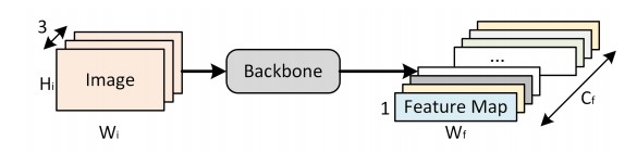
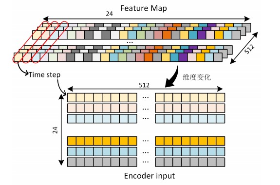
Review how the image is constructed as the input of the Transformer after it passes through the backbone:
After the image passes through the backbone, a feature map with dimension [batch_size,512,1,24] will be output. If you don't pay attention to batch_ On the premise of size, each image will get 1 with 512 channels as shown below × 24, as shown in the red box in the figure, the eigenvalues at the same position of different channels are spliced to form a new vector and used as the input of a time step. At this time, the input with dimension [batch_size, 24512] is constructed to meet the input requirements of Transformer.
model structure
class OCR_EncoderDecoder(nn.Module):
'''
A standard Encoder-Decoder architecture.
Base for this and many other models.
'''
 def __init__(self,encoder,decoder,src_embed,src_position,tgt_embed,generator):
   super(OCR_EncoderDecoder,self).__init__()
   self.encoder=encoder
   self.decoder=decoder
   self.src_embed=src_embed #input embedding module
   self.src_position=src_position
   self.tgt_embed=tgt_embed #output embedding mudule
   self.generator=generator #output generation module

 def forward(self,src,tgt,src_mask,tgt_mask):
   "Take in and process masked src and target sequences."
   #src-->[bs,3,32,768] [bs,c,h,w]
   #src_mask -->[bs,1,24] [bs,h/32,w/32]
   memory=self.encode(src,src_mask)
   #memory-->[bs,24,512]
   #tgt-->decode_in[bs,20] [bs,sequence_len-1]
   #tgt_mask-->decode_mask [bs,20] [bs,sequence_len-1]
   res=self.decode(memory,src_mask,tgt,tgt_mask) #[bs_20,512]
   return res

def encode(self,src,src_mask):
   #feature extract
   #src-->[bs,3,32,768]
   src_embedds=self.src_embed(src)
   #resnet18 is used here as the backbone output -- > [batchsize, C, h, w] -- > [BS, 512,1,24]
   #Set src_embedds is processed by shape(bs,model_dim,1,max_ratio) into the input shape(bs, time step, model_dim) expected by the transformer
   #[bs,512,1,24]-->[bs,24,512]
   src_embedds=src_embedds.squeeze(-2)
   src_embedds=src_embedds.permute(0,2,1)

   #position encode
   src_embedds=self. src_position(src_embedds) #[bs,24,512]
   return self.encoder(src_embedds,src_mask) #[bs,24,512]

def decode(self,memory,src_mask,tgt,tgt_mask):
   target_embedds=self.tgt_embed(tgt) #[bs,20,512]
   return self.decoder(targget_embedds,memory,src_mask,tgt_mask)

def make_ocr_model(tgt_vocab,N=6,d_model=512,d_ff=2048,h=8,dropout=0.1):
'''
Build model
params:
  tgt_vocab:Output dictionary size
  N:Number of encoder and decoder stack base modules
  d_model:In the model embedding of size,The default is 512
  d_ff:FeedForward Layer In layer embedding of size,The default is 2048
  h:MultiHeadAttention The number of multiple heads in must be d_model to be divisible by
  dropout: dropout Ratio of
'''
  c=copy.deepcopy

 #resnet18 pre trained in torch is used as feature extraction network, backbone
 backbone=models.resnet18(pretrained=True)
 backbone=nn.Sequential(*list(backbone.children())[:-2]) #Remove the last two layers (global average pooling and fc layer)

 attn=MultiHeadedAttention(h,d_model)
 ff=PositionwiseFeedForward(d_model,d_ff,dropout)
 position=PostionalEncoding(d_model,dropout)
 #Build model
 model=OCR_EncoderDecoder(
     Encoder(EncoderLayer(d_model,c(attn),c(ff),dropout),N),
     Decoder(DecoderLayer(d_model,c(attn),c(attn),c(ff),dropout),N),
     backbone,
     c(position),
     nn.Sequential(Embeddings(d_model,tgt_vocab),c(position)),
     Generator(d_model,tgt_vocab)) #The generator here is not called inside the class

#Initialize parameters with Glorot/fan_avg.
for child in model.children():
   if child is backbone:
    #Set the weight of the backbone to not calculate the gradient
      for param in child.parameters():
           param.requires_grad=False
    #The pre trained backbone is not initialized randomly, and the other modules are initialized randomly
      continue
   for p in child.parameters():
      if p.dim()>1:
          nn.init.xavier_uniform_(p)
   return model
The transformer model can be easily built through the above two classes:
transformer model
#build model
#use transformer as ocr recognize model
#OCR built here_ The model does not contain a Generator
tgt_vocab=len(lbl2id_map.keys())
d_model=512
ocr_model=make_ocr_model(tgt_vocab,N=5,d_model=d_model,d_ff=2048,h=8,dropout=0.1)
ocr_model.to(device)
4. Model training
Before model training, we also need to define model evaluation criteria, iterative optimizer, etc. During the training of this experiment, strategies such as label smoothing and network training warm-up are used. [the calling function is in the train_utils.py file]
Label smoothing can convert the original hard label into soft label, so as to increase the fault tolerance of the model and improve the generalization ability of the model. The * * LabelSmoothing() function in the code implements label smoothing, and the relative entropy function is used internally to calculate the loss between the predicted value and the real value.
The warmup strategy can effectively control the learning rate of the optimizer in the process of model training, and automatically realize the control of the model learning rate from small increase to gradual decrease, which helps the model to be more stable during training and realize the rapid convergence of loss. The noamot() * * function in the code realizes the warmup control, and the Adam optimizer is used to realize the automatic adjustment of the number of iterations of the learning rate.
Label smoothing before model training and network training warm-up are implemented
#train prepare
criterion=LabelSmoothing(size=tgt_vocab,padding_idx=0,smoothing=0.0) #label smoothing
optimizer=torch.optim.Adam(ocr_model.parameters(),lr=0,betas=(0.9,0.98),eps=1e-9)
model_opt=NoamOpt(d_model,1,400,optimizer) #warmup
The code of the model training process is as follows. Every 10 epochs are trained for verification. The calculation process of a single epoch is encapsulated in the * * run_epoch() * * function.
#train&valid...
for epoch in range(nrof_epochs):
    print(f"\nepoch {epoch}")

   print("train...") #train
   ocr_model.train()
   loss_compute=SimpleLossCompute(ocr_model.generator,criterion,model_opt)
   train_mean_loss=run_epoch(train_loader,ocr_model,loss_compute,device)
   if epoch %10 ==0 :
     print("valid...") #verification
     ocr_model.eval()
     valid_loss_compute=SimpleLossCompute(ocr_model.generator,criterion,None)
     valid_mean_loss=run_epoch(valid_loader,ocr_model,valid_loss_compute,device)
     print(f"valid loss:{valid_mean_loss}")

    #save model
    torch.save(ocr_model.state_dict(),'./trained_model/ocr_model.pt')
The SimpleLossCompute() class implements the loss calculation of transformer output results. When using this class for direct calculation, the class needs to accept (x,y,norm) Three parameters, X is the output result of the decoder, y is the label data, norm is the normalization coefficient of loss, and the number of all valid token s in batch can be used. It can be seen that the construction of all networks of the transformer is being completed here to realize the flow of data calculation flow.
The run_epoch() function completes all the work of epoch training, including data loading, model reasoning, loss calculation and direction propagation, and prints the training process information.
def run_epoch(data_loader,model,loss_compute,device=None):
"Standard Training and Logging Function"
    start=time.time()
    total_tokens=0
    total_loss=0
    tokens=0

    for i ,batch in enumerate(data_loader):
        img_input,encode_mask,decode_in,decode_out,decode_mask,ntokens=batch
        img_input=img_input.to(device)
        encode_mask=encode_mask.to(device)
        decode_in=decode_in.to(device)
        decode_out=decode_out.to(device)
        decode_mask=decode_mask.to(device)
        ntokens=torch.sum(ntokens).to(device)

        out=model.forward(img_input,decode_in,encode_mask,decode_mask)
        #Out -- > [BS, 20512] forecast results
        #Decode_out -- > [BS, 20] actual results
        #Actual valid characters in tokens -- > tag

        loss=loss_compute(out,decode_out,ntokens)#Loss calculation
        total_loss+=loss
        total_tokens+=ntokens
        tokens+=ntokens
        if i % 50 ==1:
           elapsed=time.time()-start
           print("Epoch Step: %d Loss:%f Tokens per Sec:%f"%(i,loss/ntokens,tokens/elapsed))
           start=time.time()
           tokens=0
return total_loss/total_tokens

class SimpleLossCompute:
   "A simple loss compute and train function."
   def __init__(self,generator,criterion,opt=None):
      self.generator=generator
      self.criterion=criterion
      self.opt=opt

   def __call__(self,x,y,norm):
   '''
   norm:loss Normalization coefficient of, using batch All valid in token Just count
   '''
   #X -- > out -- > [BS, 20512] forecast results
   #Y -- > decode_out -- > [BS, 20] actual results
   #Actual valid characters in Norm -- > tokens -- > tag
   x=self.generator(x)
   #label smoothing needs to correspond to dimension changes
   x_=x.contiguous().view(-1,x.size(-1)) #[20bs,512]
   y_=y.contiguous().view(-1) #[20bs]
   loss=self.criterion(x_,y_)
   loss /=norm
   loss.backward()
   if self.opt is not None:
      self.opt.step()
      self.opt.optimizer.zero_grad()
   #return loss.data[0]*norm
   return loss.item()*norm
5. Greedy decoding
We use the simplest greedy decoding to predict the OCR result directly. Because the model will only produce one output at a time, we select the character corresponding to the highest probability in the output probability distribution as the prediction result, and then predict the next character, which is the so-called greedy decoding.
In the experiment, each image is used as the input of the model, greedy decoding is carried out one by one, and the prediction accuracy of the training set and the verification set is finally given.
Greedy decoding
#After the training, the greedy decoding method is used to infer the training set and verification set, and the accuracy is counted
ocr_model.eval()

print('\n-----------------------------------------------')
print("greedy decode trainset")
total_img_num=0
total_correct_num=0
for batch_idx,batch in enumerate(train_loader):
   img_input,encode_mask,decode_in,decode_out,decode_mask,ntokens=batch
   img_input=img_input.to(device)
   encode_mask=encode_mask.to(device)

   #Get single image information
   bs=img_input.shape[0]
   for i in range(bs):
       cur_img_input=img_input[i].unsqueeze(0)
       cur_encode_mask=encode_masl[i].unsqueeze(0)
       cur_decode_out=decode_out[i]
       #Greedy decoding
       pred_result=greedy_decode(ocr_model,cur_img_input,cur_encode_mask,max_len=sequence_len,start_symbol=1,end_symbol=2)
       pred_result=pred_result.cpu()
       #Judge whether the prediction is correct
       is_correct=judge_is_correct(pred_result,cur_decode_out)
       total_correct_num+=is_correct
       total_img_num+=1
       if not is_correct:
           #Print case with wrong prediction
           print("----")
           print(cur_decode_out)
           print(pred_result)
       total_correct_rate=total_correct_num/total_img_num*100
       print(f"total correct rate of trainset:{total_correct_rate}%")

#Same as training set decoding code
print("\n----------------------------")
print("greedy decode validset")
total_img_num=0
total_correct_num=0
for batch_idx,batch in enumerate(valid_loader):
    img_input,encode_mask,decode_in,decode_out,decode_mask,ntokens=batch
    img_input=img_input.to(device)
    encode_mask=encode_mask.to(device)

    bs=img_input.shape[0]
    for i in range(bs):
       cur_img_input=img_input[i].unsqueeze(0)
       cur_encode_mask=encode_mask[i].unsqueeze(0)
       cir_decode_out=decode_out[i]

       pred_result=greedy_decode(ocr_model,cur_img_input,cur_encode_mask,max_len=sequence_len,start_symbol=1,end_symbol=2)
       pred_result=pred_result.cpu()

       is_correct=judge_is_correct(pred_result,cur_decode_out)
       total_correct_num+=is_correct
       total_img_num+=1
       if not is_correct:
          #Print case of forecast data
          print("----")
          print(cur_decode_out)
          print(pred_result)
       total_correct_rate=total_correct_num/total_img_num*100
       print(f"total correct rate of validset:{total_correct_rate}%")
greedy decode
#greedy decode
def greedy_decode(model,src,src_mask,max_len,start_symbol,end_symbol):
  memory=model.encode(src,src_mask)
  #ys represents the currently generated sequence. Initially, it is a sequence containing only one starting character, and the prediction result is continuously appended to the end of the sequence
  ys=torch.ones(1,1).fill_(start_symbol).type_as(src.data).lo ng()
  for i in range(max_len-1):
       out=model.decode(memory,src_mask,Variable(ys),Variable(subsequent_mask(ys.size(1)).type_as(src.data)))
       prob=model.generator(out[:-1])
       _,next_word=torch.max(prob,dim=1)
       new_word=next_word.data[0]
       next_word=torch.ones(1,1).type_as(src.data).fill_(next_word).long()
       ys=torch.cat([ys,next_word],dim=1)
       next_word=int(next_word)
       if next_word==end_symbol:
           break
       #ys=torch.cat([ys,torch.ones(1,1).type_as(src.data).fill_(next_word)],dim=1)
  ys=ys[0,1:]
  return ys

def judge_is_correct(pred,label):
    #Judge whether the predicted results of the model are consistent with the label
    pred_len=pred.shape[0]
    label=label[:pred_len]
    is_correct=1 if label.equal(pred) else 0
    return is_correct