https://github.com/vqv/ggbiplot/blob/master/README.md
A few days ago in the "Macro Genome 0" Wechat discussion group saw someone send a link above, click on it to see that it is actually a command map, it is very practical. I immediately used the OTU table in this field to test, the effect is very good, now share with you, welcome to leave a message to supplement.
Introduction to ggbiplot
ggbiplot is a R package tool for visualizing the results of PCA analysis. ggplot2 can be directly used to visualize the results of prcomp() PCA analysis of the basic function in R. It can also be grouped by coloring, adding ellipses of different sizes, correlation and contribution vectors between principal components and original variables.
An implementation of the biplot using ggplot2. The package provides two functions: ggscreeplot() and ggbiplot(). ggbiplot aims to be a drop-in replacement for the built-in R function biplot.princomp() with extended functionality for labeling groups, drawing a correlation circle, and adding Normal probability ellipsoids.
ggbiplot installation and official examples
R package, more convenient to use in Rstudio
# Installation Package, Installation Over Please Skip
install.packages("devtools", repo="http://cran.us.r-project.org")
library(devtools)
install_github("vqv/ggbiplot")

# The simplest and most handsome example
data(wine)
wine.pca <- prcomp(wine, scale. = TRUE)
# Demo Style
ggbiplot(wine.pca, obs.scale = 1, var.scale = 1,
         groups = wine.class, ellipse = TRUE, circle = TRUE) +
  scale_color_discrete(name = '') +
  theme(legend.direction = 'horizontal', legend.position = 'top')


# basic style
plot(wine.pca$x) # The original picture, you can try to draw, can not bear to look directly at- 1
- 2
- 3
- 4
- 5
- 6
- 7
- 8
- 9
- 10
- 11
- 12
- 13
- 14
- 15
- 16
- 17
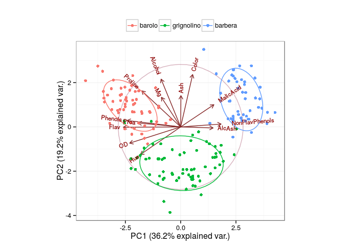
See, is it a command to show the results of principal component analysis PCA obtained by prcomp() incisively and vividly? Is there a high score article B in a flash?
The main results show that:
- The value of coordinate axis PC1/2 is the explanatory rate of the overall difference.
- The dots in the picture represent samples, the colors represent groups, and the legends have three groups at the top.
- The ellipse represents the core area added by the default confidence interval of 68%, which facilitates the separation between the observation groups.
- The arrow represents the original variable, in which the direction represents the correlation between the original variable and the principal component, and the length represents the contribution of the original data to the principal component.
More detailed PCA principles, derivations, diagrams, please jump "Understanding PCA Principal Component Analysis in One Paper" Then Click to read the original text. Focus on the interpretation of PCA results.
OTU Tables in Practice
This battle, based on the publication of articles before this public number Amplifier Analysis Course-3 Statistical Mapping-Impact High Score Articles The OTU table, experimental design and species annotation information of the test data can be downloaded if needed.
PCA Analysis of OTU Tables and Visualization
# Microbial Data Actual Combat
# Read-in experiment design
design = read.table("design.txt", header=T, row.names= 1, sep="\t")

# Read OTU table
otu_table = read.delim("otu_table.txt", row.names= 1,  header=T, sep="\t")

# Filtering data and sorting
idx = rownames(design) %in% colnames(otu_table)
sub_design = design[idx,]
count = otu_table[, rownames(sub_design)]

# PCA Analysis Based on OTU Table
otu.pca <- prcomp(t(count), scale. = TRUE)

# Draw PCA diagram and add ellipses by group
ggbiplot(otu.pca, obs.scale = 1, var.scale = 1,
groups = sub_design$genotype, ellipse = TRUE,var.axes = F)- 1
- 2
- 3
- 4
- 5
- 6
- 7
- 8
- 9
- 10
- 11
- 12
- 13
- 14
- 15
- 16
- 17
- 18
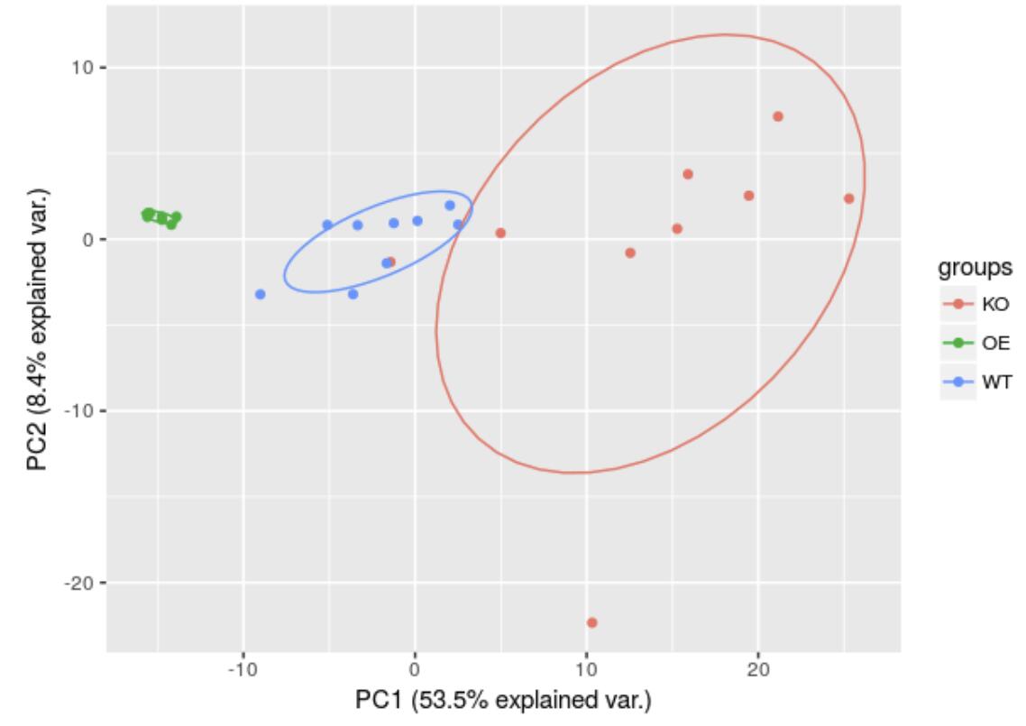
It can be seen that the three groups are distinctly separated on the first spindle.
Demonstrating the relationship between the main differentiated bacteria and the principal components
# Effect of Significant High Abundance Bacteria

# Convert raw data to percentage
norm = t(t(count)/colSums(count,na=T)) * 100 # normalization to total 100

# Screening OTU with mad value greater than 0.5
mad.5 = norm[apply(norm,1,mad)>0.5,]
# Another method: rank OTUs with the highest volatility in the first six by mad value
mad.5 = head(norm[order(apply(norm,1,mad), decreasing=T),],n=6)
# Calculating the correlation between PCA and bacterial axis
otu.pca <- prcomp(t(mad.5))
ggbiplot(otu.pca, obs.scale = 1, var.scale = 1,
groups = sub_design$genotype, ellipse = TRUE,var.axes = T)- 1
- 2
- 3
- 4
- 5
- 6
- 7
- 8
- 9
- 10
- 11
- 12
- 13
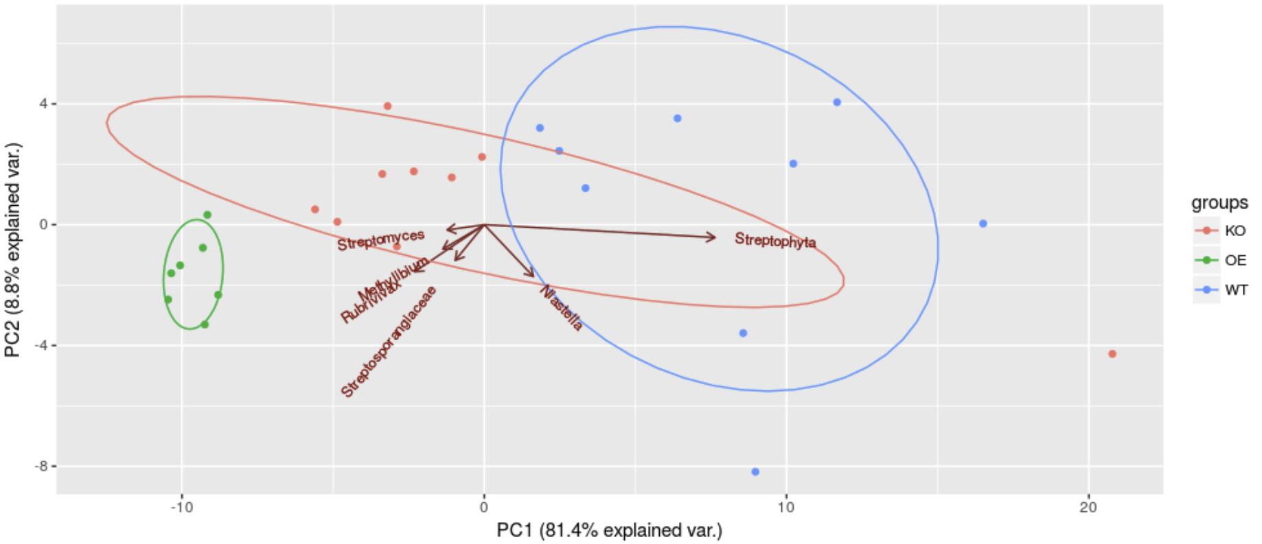
We can clearly separate the three groups of samples by principal component analysis using only six OTUs with the largest median absolute deviation (mad). The length of vectors in the graph represents the difference contribution, and the direction is the correlation with the principal component. It can be seen that the longest vector Streptophyta is nearly parallel to the X axis, indicating that the difference of PC1 is mainly due to the bacterial contribution. Other bacteria may negatively correlate with OTUs in the opposite direction, and those with angle less than 90% have a positive correlation with OTUs.
Introduction to ggbiplot official website
ggbiplot
An implementation of the biplot using ggplot2. The package provides two functions: ggscreeplot() and ggbiplot(). ggbiplot aims to be a drop-in replacement for the built-in R function biplot.princomp() with extended functionality for labeling groups, drawing a correlation circle, and adding Normal probability ellipsoids.
ggbiplot usage and parameters
?ggbiplot

ggbiplot(pcobj, choices = 1:2, scale = 1, pc.biplot =
  TRUE, obs.scale = 1 - scale, var.scale = scale, groups =
  NULL, ellipse = FALSE, ellipse.prob = 0.68, labels =
  NULL, labels.size = 3, alpha = 1, var.axes = TRUE, circle
  = FALSE, circle.prob = 0.69, varname.size = 3,
  varname.adjust = 1.5, varname.abbrev = FALSE, ...)

pcobj # prcomp() or princomp() returns the result
choices # Select axis, default 1:2
scale   # covariance biplot (scale = 1), form biplot (scale = 0). When scale = 1, the inner product between the variables approximates the covariance and the distance between the points approximates the Mahalanobis distance.
obs.scale # Standardized observations
var.scale # Standardized variation
pc.biplot # Compatible with biplot.princomp()
groups # Group information and colour by group
ellipse # Adding group ellipses
ellipse.prob # confidence interval
labels  # Vector name
labels.size # Name size
alpha # Point transparency (0 = TRUEransparent, 1 = opaque)
circle # Draw the correlation ring (only apply when prcomp was called with scale = TRUE and when var. scale = 1)
var.axes # Drawing Line-Bacteria Relationships of Variables
varname.size # Variable name size
varname.adjust # Distance between label and arrow >= 1 means farther from the arrow
varname.abbrev # Whether the label is abbreviated or not- 1
- 2
- 3
- 4
- 5
- 6
- 7
- 8
- 9
- 10
- 11
- 12
- 13
- 14
- 15
- 16
- 17
- 18
- 19
- 20
- 21
- 22
- 23
- 24
- 25
- 26
Guess you like it
- Read a passage: 1 Microbiome 2 evolutionary tree 3. Predicting community function
- Hot text: 1 Chart Specification 2 DNA Extraction 3 experimental vs analysis
- Essential skills: 1 Questions 2 Search 3Endnote
- Literature Reading 1 Warmhearted 2SemanticScholar 3geenmedical
- Amplifier analysis: 1 Chart Interpretation 2 Analysis process 3. Statistical mapping 4 Community Functions 5 evolutionary tree
- Scientific research team experience: 1 Cloud Notebook 2 Cloud Collaboration 3 Public Number
- Series of Courses: 1Biostar 2 Microbiome 3 macrogenome
- Popularization of Biology Science 1 Intestinal bacteria 2 Great Leap Forward of Life 3-Cell Secret Warfare 4 Human Mysteries