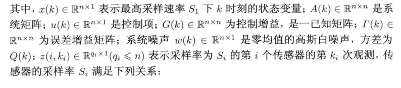
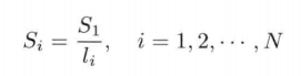
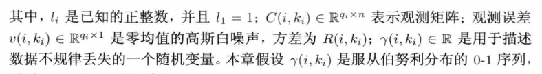
Problem description
There are N sensors for observation, and there is a certain probability that the observation data will be lost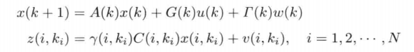
In short, where γ \ gamma γ is a random number (non-zero is 1), 0 represents data loss, and 1 represents data existence. Other multi-sensor and multi rate representations are consistent with the previous article.
The following also rewrites the multi rate model into a single model.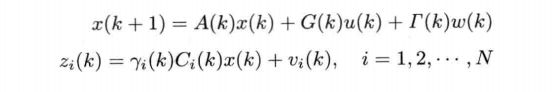
among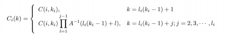
Algorithm deduction
The derivation of the reconstruction parameters of the state transition equation of multi-rate and multi-sensor has been described in detail in the previous paper. Here, only the observation equation, i.e. different parts, are discussed.
In order to simplify the derivation of the state transition equation, the control term is set to 0, and the noise gain matrix γ \ Gamma γ is set to the unit matrix, that is, x(k+1)=A(k)x(k)+w(k) + X (k) + x(k+1)=A(k)x(k)+w(k) x (K + 1) = a (k) x (k) + W (k)
In the same way, we can write: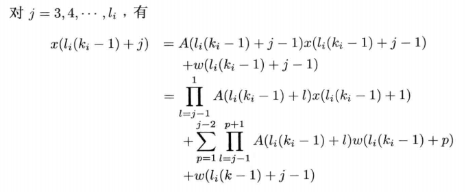 At this time, move x (l i (ki − 1) + 1) \ x (L ﹣ I (K ﹣ i-1) + 1) x(li(ki − 1) + 1) to the left
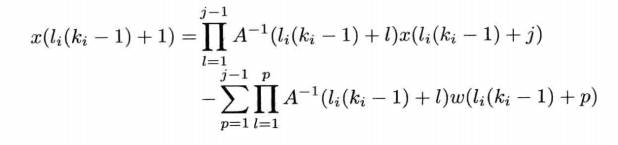
Then according to the observation equation, we can get: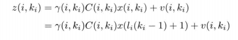
By substituting the state transfer equation derived above into the observation equation, we can get:
- x (l i (ki − 1)+j)\ I (k i-1) + 1) z(li(ki − 1) + 1) is corrected (as can be seen from Ci \ C CI).
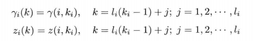
Here, we can see the parameters of the reconstructed observation equation. On the right side of the equation, the first term is γ (i,ki)Cix(li(ki − 1)+j), gamma (I, K } I) C } I x (L } i-1)+j) γ (i,ki) Ci x(li (ki − 1) + J, and the sum of the second term and the third term is vi (k) \ V } I (k) vi (k)
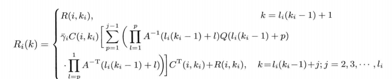
According to these two parameters, we can deduce the reconstruction parameters Ci, Ri \ C, R \ i ci, Ri given in the problem description
If the state transition matrix is not simplified, what are the parameters of reconstruction?
Fusion algorithm


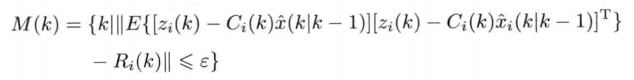
The M(k) m (k) M(k) m (k) set here is actually a set of lost data times. How to understand the mathematical description of the above set? Personal understanding: data loss means that it can not filter and correct the predicted data. From the set, we can see that E{[zi(k) - Ci(k)x^(k ∣ K − 1)][zi(k) - Ci(k)x^(k ∣ K − 1)]T}\ Noise matrix, because in the sense of probability, the mean value of the observed value and the predicted value is regarded as the true value, but the actual data are all samples In terms of probability distribution, the above formula can be regarded as the variance of a probability distribution whose mean value is 0. If the variance is infinitely close to the observation noise matrix Ri \ R ﹤ Ri of the sensor, then it means that the correction effect of the deviation between the observation value and the predicted value is covered by the observation noise of the sensor, and the filtering correction effect is lost, reflecting the data loss.
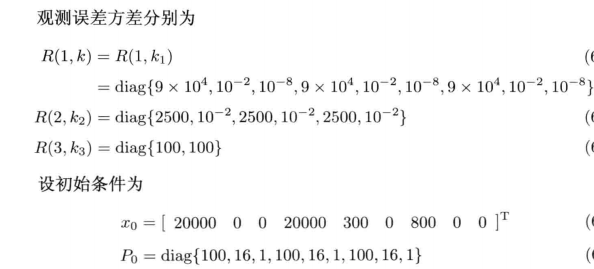
Simulation example
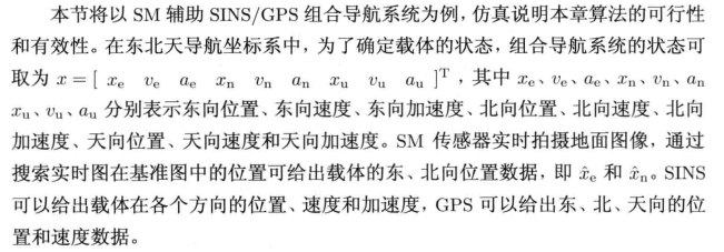
Set u(k)=0, γ (k) = IU (k) = 0, gamma (k) = IU (k) = 0, γ (k) = isins, GPS and SM as sensors 1, 2 and 3 respectively.
Observation matrix:


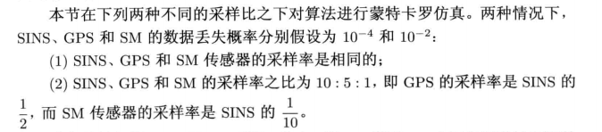
The second case is simulated by the program here. For the setting of this simulation, the RI (k) r UUI (k) RI (k) derived from the simplified model can be used
%%%===========Robust fusion design of multi rate sensors with random packet loss========%%%
clc;
clear all;
close all;
%% Data generation
%Let an aircraft fly at a fixed altitude at approximately uniform acceleration(Assume the direction is northeast)
%State matrix x by9x1   The states are respectively in the east direction/Eastward velocity/East acceleration/Northward position/Northward velocity/North acceleration/Direction of heaven/Radial velocity/Celestial acceleration
%x=[xe ve ae xn vn an xu vu au]';
%Generate the actual flight data. The flight acceleration is5m/s^2
N=500;%time span
n1=1;      %SINS Sampling interval
n2=2;      %GPS Sampling interval
n3=10;     %SM Sampling interval
M=lcm(n2,n3);%The minimum common multiple of sampling interval is the fusion period
M1=M/n1;
M2=M/n2;
M3=M/n3;
t=1:1:N ;  %time series
X0=[0 0 0 0 300 0 800 0 0 ];%Initial state
P0=diag([100,16,1,100,16,1,100,16,1]);
%Actual data
xe=0.5*5*0.707*t.^2;
ve=5*0.707*t;
ae=5*0.707*ones(1,N);
xn=300*t+0.5*5*0.707*t.^2;
vn=300+5*0.707*t;
an=5*0.707*ones(1,N);
xu=800*ones(1,N);
vu=zeros(1,N);
au=zeros(1,N);
%Generation of observation data
%1.Simultaneous interpreting noise due to different sensor pairs/The measurement noise of velocity and acceleration is not the same, so noise is added one by one.
%SINS Northeast celestial position/speed/Acceleration inertial navigation
SINS_xe=xe+randn(1,N)*sqrt(90000);
SINS_ve=ve+randn(1,N)*sqrt(0.01);
SINS_ae=ae+randn(1,N)*sqrt(10^-8);
SINS_xn=xn+randn(1,N)*sqrt(90000);
SINS_vn=vn+randn(1,N)*sqrt(0.01);
SINS_an=an+randn(1,N)*sqrt(10^-8);
SINS_xu=xu+randn(1,N)*sqrt(90000);
SINS_vu=vu+randn(1,N)*sqrt(0.01);
SINS_au=au+randn(1,N)*sqrt(10^-8);
%GPS Northeast celestial position/speed
GPS_xe=xe+randn(1,N)*sqrt(2500);
GPS_ve=ve+randn(1,N)*sqrt(0.01);
GPS_xn=xn+randn(1,N)*sqrt(2500);
GPS_vn=vn+randn(1,N)*sqrt(0.01);
GPS_xu=xu+randn(1,N)*sqrt(2500);
GPS_vu=vu+randn(1,N)*sqrt(0.01);
%SM Scene matching northeast position data
SM_xe=xe+randn(1,N)*sqrt(100);
SM_xn=xn+randn(1,N)*sqrt(100);

%observed data
%SINS
SINS_z=cell(9,1);
SINS_z(1,1)={SINS_xe};
SINS_z(2,1)={SINS_ve};
SINS_z(3,1)={SINS_ae};
SINS_z(4,1)={SINS_xn};
SINS_z(5,1)={SINS_vn};
SINS_z(6,1)={SINS_an};
SINS_z(7,1)={SINS_xu};
SINS_z(8,1)={SINS_vu};
SINS_z(9,1)={SINS_au};
SINS_z=cell2mat(SINS_z);
%GPS
GPS_z=cell(6,1);
GPS_z(1,1)={GPS_xe};
GPS_z(2,1)={GPS_ve};
GPS_z(3,1)={GPS_xn};
GPS_z(4,1)={GPS_vn};
GPS_z(5,1)={GPS_xu};
GPS_z(6,1)={GPS_vu};
GPS_z=cell2mat(GPS_z);
%SM
SM_z=cell(2,1);
SM_z(1,1)={SM_xe};
SM_z(2,1)={SM_xn};
SM_z=cell2mat(SM_z);
%% transition matrix/Observation matrix/Noise matrix/     Sparse matrix can be used here to save memory A=sparse(r,c,S)
%transition matrix
A=[1 1 0.5 0 0 0 0 0 0
    0 1 1 0 0 0 0 0 0
    0 0 1 0 0 0 0 0 0
    0 0 0 1 1 0.5 0 0 0
    0 0 0 0 1 1 0 0 0
    0 0 0 0 0 1 0 0 0
    0 0 0 0 0 0 1 1 0.5
    0 0 0 0 0 0 0 1 1
    0 0 0 0 0 0 0 0 1];
%Observation matrix
C1=eye(9);
C2=[1 0 0 0 0 0 0 0 0
    0 1 0 0 0 0 0 0 0
    0 0 0 1 0 0 0 0 0
    0 0 0 0 1 0 0 0 0
    0 0 0 0 0 0 1 0 0
    0 0 0 0 0 0 0 1 0];
C3=[1 0 0 0 0 0 0 0 0
    0 0 0 1 0 0 0 0 0];
%Noise matrix
R1=diag([90000 0.01 10^-8  90000 0.01 10^-8  90000 0.01 10^-8]);
R2=diag([2500 0.01 2500 0.01 2500 0.01]);
R3=diag([100 100]);
Q=(A^2)*5;

%% Wave filtering
%Suppose that the time when three sensors get data synchronously is i=1,i=11......501
X=cell(1,501);
X(1)={X0'};
for i=1:N

    if rem(i-1,n2)==0
        if rem(i-1,n3)==0
           %In this case, all three sensors get data
           %Random loss number generation
           shadow1=rand(1,1);
           shadow2=rand(1,1);
           shadow3=rand(1,1);
           %Forecast
           temp=A*cell2mat(X(i));
           P1=A*P0*A'+Q;
  %Data loss judgment
         if shadow1<0.0001   %The probability of loss is10^-4
             K1=zeros(9,9);
         else
             K1=P1*C1'/(C1*P1*C1'+R1);
         end
         if shadow2<0.0001   %The probability of loss is10^-4
             K2=zeros(9,6);
         else
             K2=P1*C2'/(C2*P1*C2'+R2);

         end
          if shadow3<0.01   %The probability of loss is10^-2
             K3=zeros(9,2);
         else
             K3=P1*C3'/(C3*P1*C3'+R3);

         end
 %K It's worth it
 %Estimate
          x1=temp+K1*(SINS_z(:,i)-C1*temp);
          x2=temp+K2*(GPS_z(:,i)-C2*temp);
          x3=temp+K3*(SM_z(:,i)-C3*temp);
          p1=(eye(9,9)-K1*C1)*P1;
          p2=(eye(9,9)-K2*C2)*P1;
          p3=(eye(9,9)-K3*C3)*P1;
          p_1=inv(p1);
          p_2=inv(p2);
          p_3=inv(p3);
 %Fusion
         P0=inv(p_1+p_2+p_3);
         X(i+1)={P0*(p_1*x1+p_2*x2+p_3*x3)};

        else
           %In this case, only SINS And GPS Get data
           %Random loss number generation
           shadow1=rand(1,1);
           shadow2=rand(1,1);
            %Forecast
           temp=A*cell2mat(X(i));
           P1=A*P0*A'+Q;
           j3=rem(i-1,n3);
           %Data loss judgment
         if shadow1<0.0001   %The probability of loss is10^-4
             K1=zeros(9,9);
         else
             K1=P1*C1'/(C1*P1*C1'+R1);
         end
         if shadow2<0.0001   %The probability of loss is10^-4
             K2=zeros(9,6);
         else
             K2=P1*C2'/(C2*P1*C2'+R2);

         end
         %Get noise matrix
         %R3
         R_3=zeros(9,9);
         for n=1:j3
            R_3=(inv(A)^n)*Q*(inv(A')^n)+R_3;
         end
         R_3=0.99*C3*(inv(A)^(j3))*R_3*(C3*(inv(A)^(j3)))'+R3;
         %Gain matrix obtained
         K3=P1*(C3*(inv(A)^(j3)))'/(C3*inv(A)^(j3)*P1*(C3*(inv(A)^(j3)))'+R_3);

         %estimate
          x1=temp+K1*(SINS_z(:,i)-C1*temp);
          x2=temp+K2*(GPS_z(:,i)-C2*temp);
          x3=temp+K3*(SM_z(:,i-j3)-C3*(inv(A)^(j3))*temp);
          p1=(eye(9,9)-K1*C1)*P1;
          p2=(eye(9,9)-K2*C2)*P1;
          p3=(eye(9,9)-K3*C3*inv(A)^(j3))*P1;
          p_1=inv(p1);
          p_2=inv(p2);
          p_2=inv(p3);
%Fusion
         P0=inv(p_1+p_2+p_3);
        X(i+1)={P0*(p_1*x1+p_2*x2+p_3*x3)};
        end


    else
        if rem(i-1,n3)==0
           %In this case SINS And SM Sensor information
           %Random loss number generation
           shadow1=rand(1,1);
           shadow3=rand(1,1);
        %Forecast
           temp=A*cell2mat(X(i));
           P1=A*P0*A'+Q;
           j2=rem(i-1,n2);
            %Data loss judgment
         if shadow1<0.0001   %The probability of loss is10^-4
             K1=zeros(9,9);
         else
             K1=P1*C1'/(C1*P1*C1'+R1);
         end
          if shadow3<0.01   %The probability of loss is10^-2
             K3=zeros(9,2);
         else
             K3=P1*C3'/(C3*P1*C3'+R3);

          end
        %Get noise matrix
         %R2
         R_2=zeros(9,9);
         for n=1:j2
            R_2=(inv(A)^n)*Q*(inv(A')^n)+R_2;
         end
         R_2=0.9999*C2*(inv(A)^(j2))*R_2*(C2*(inv(A)^(j2)))'+R2;
          %Gain matrix obtained
         K2=P1*(C2*(inv(A)^(j2)))'/(C2*inv(A)^(j2)*P1*(C2*(inv(A)^(j2)))'+R_2);

          %estimate
          x1=temp+K1*(SINS_z(:,i)-C1*temp);
          x2=temp+K2*(GPS_z(:,i-j2)-C2*(inv(A)^(j2))*temp);
          x3=temp+K3*(SM_z(:,i)-C3*temp);
          p1=(eye(9,9)-K1*C1)*P1;
          p2=(eye(9,9)-K2*C2*inv(A)^(j2))*P1;
          p3=(eye(9,9)-K3*C3)*P1;
          p_1=inv(p1);
          p_2=inv(p2);
          p_2=inv(p3);
%Fusion

         P0=inv(p_1+p_2+p_3);
         X(i+1)={P0*(p_1*x1+p_2*x2+p_3*x3)};


        else
           %In this case, only SINS data
           %Random loss number generation
           shadow1=rand(1,1);
           %Forecast
           temp=A*cell2mat(X(i));
           P1=A*P0*A'+Q;
           j2=rem(i-1,n2);
           j3=rem(i-1,n3);
           %Data loss judgment
         if shadow1<0.0001   %The probability of loss is10^-4
             K1=zeros(9,9);
         else
             K1=P1*C1'/(C1*P1*C1'+R1);
         end
         %Get noise matrix
         %R2
         R_2=zeros(9,9);
         for n=1:j2
            R_2=(inv(A)^n)*Q*(inv(A')^n)+R_2;
         end
         R_2=0.9999*C2*(inv(A)^(j2))*R_2*(C2*(inv(A)^(j2)))'+R2;
         %R3
         R_3=zeros(9,9);
         for n=1:j3
            R_3=(inv(A)^n)*Q*(inv(A')^n)+R_3;
         end
         R_3=0.99*C3*(inv(A)^(j3))*R_3*(C3*(inv(A)^(j3)))'+R3;
         %Gain matrix obtained
         K2=P1*(C2*(inv(A)^(j2)))'/(C2*inv(A)^(j2)*P1*(C2*(inv(A)^(j2)))'+R_2);

         K3=P1*(C3*(inv(A)^(j3)))'/(C3*inv(A)^(j3)*P1*(C3*(inv(A)^(j3)))'+R_3);

         %estimate
          x1=temp+K1*(SINS_z(:,i)-C1*temp);
          x2=temp+K2*(GPS_z(:,i-j2)-C2*(inv(A)^(j2))*temp);
          x3=temp+K3*(SM_z(:,i-j3)-C3*(inv(A)^(j3))*temp);
          p1=(eye(9,9)-K1*C1)*P1;
          p2=(eye(9,9)-K2*C2*inv(A)^(j2))*P1;
          p3=(eye(9,9)-K3*C3*inv(A)^(j3))*P1;
          p_1=inv(p1);
          p_2=inv(p2);
          p_2=inv(p3);
%Fusion
         P0=inv(p_1+p_2+p_3);
       X(i+1)={P0*(p_1*x1+p_2*x2+p_3*x3)};
        end
    end
end

%% Image rendering
l=1:1:500;
X=cell2mat(X);
X=X(1:9,2:501);
%Actual vs. estimated
subplot(3,1,1)
plot(l,X(1,:),'b',l,xe,'r');
title('Eastward position');
legend('Estimated value','actual value');
xlabel('t');
ylabel('s');
subplot(3,1,2)
plot(l,X(2,:),'b',l,ve,'r');
title('Eastward velocity');
legend('Estimated value','actual value');
xlabel('t');
ylabel('v');
subplot(3,1,3)
plot(l,X(3,:),'b',l,ae,'r');
title('East acceleration');
legend('Estimated value','actual value');
xlabel('t');
ylabel('a');
figure(2)
subplot(3,1,1)
plot(l,X(4,:),'b',l,xn,'r');
title('Northward position');
legend('Estimated value','actual value');
xlabel('t');
ylabel('s');
subplot(3,1,2)
plot(l,X(5,:),'b',l,vn,'r');
title('Northward velocity');
legend('Estimated value','actual value');
xlabel('t');
ylabel('v');
subplot(3,1,3)
plot(l,X(6,:),'b',l,an,'r');
title('North acceleration');
legend('Estimated value','actual value');
xlabel('t');
ylabel('a');
figure(3)
subplot(3,1,1)
plot(l,X(7,:),'b',l,xu,'r');
title('Direction of heaven');
legend('Estimated value','actual value');
xlabel('t');
ylabel('s');
subplot(3,1,2)
plot(l,X(8,:),'b',l,vu,'r');
title('Radial velocity');
legend('Estimated value','actual value');
xlabel('t');
ylabel('v');
subplot(3,1,3)
plot(l,X(9,:),'b',l,au,'r');
title('Celestial acceleration');
legend('Estimated value','actual value');
xlabel('t');
ylabel('a');

%error
figure(4)
subplot(3,1,1)
plot(l,X(1,:)-xe,'r');
title('Absolute error of East position');
xlabel('t');
ylabel('δ');
subplot(3,1,2)
plot(l,X(2,:)-ve,'r');
title('Absolute error of East velocity');
xlabel('t');
ylabel('δ');
subplot(3,1,3)
plot(l,X(3,:)-ae,'r');
title('Absolute error of acceleration in east direction');
xlabel('t');
ylabel('δ');

figure(5)
subplot(3,1,1)
plot(l,X(4,:)-xn,'r');
title('Absolute error of North position');
xlabel('t');
ylabel('δ');
subplot(3,1,2)
plot(l,X(5,:)-vn,'r');
title('Absolute error of northward velocity');
xlabel('t');
ylabel('δ');
subplot(3,1,3)
plot(l,X(6,:)-an,'r');
title('North acceleration absolute error');
xlabel('t');
ylabel('δ');

figure(6)
subplot(3,1,1)
plot(l,X(7,:)-xu,'r');
title('Absolute error of celestial position');
xlabel('t');
ylabel('δ');
subplot(3,1,2)
plot(l,X(8,:)-vu,'r');
title('Absolute error of celestial velocity');
xlabel('t');
ylabel('δ');
subplot(3,1,3)
plot(l,X(9,:)-au,'r');
title('Absolute error of celestial acceleration');
xlabel('t');
ylabel('δ');

